Logic Synthesis Minimization of Boolean logic Technologyindependent mapping

Logic Synthesis • Minimization of Boolean logic – Technology-independent mapping • Objective: minimize # of implicants, # of literals, etc. • Not directly related to precise technology (# transistors), but correlated – consistent with objectives for any technology – Technology-dependent mapping • Linked to precise technology/library • Technology-independent mapping – Two-level minimization – sum of products (SOP)/product of sums (POS) • Karnaugh maps – “visual” technique • Quine-Mc. Cluskey method – algorithmic • Heuristic minimization – fast and “pretty good, ” but not exact – Multi-level minimization

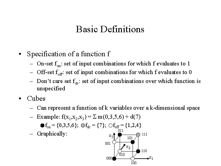
Basic Definitions • Specification of a function f – On-set fon: set of input combinations for which f evaluates to 1 – Off-set foff: set of input combinations for which f evaluates to 0 – Don’t care set fdc: set of input combinations over which function is unspecified • Cubes – Can represent a function of k variables over a k-dimensional space – Example: f(x 1, x 2, x 3) = m(0, 3, 5, 6) + d(7) fon = {0, 3, 5, 6}; – Graphically: fdc = {7}; foff = {1, 2, 4} x 3 011 101 000 x 2 111 110 010 x 1 100

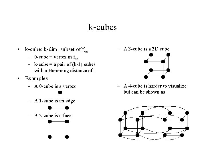
k-cubes • k-cube: k-dim. subset of fon – A 3 -cube is a 3 D cube – 0 -cube = vertex in fon – k-cube = a pair of (k-1) cubes with a Hamming distance of 1 • Examples – A 0 -cube is a vertex – A 1 -cube is an edge – A 2 -cube is a face – A 4 -cube is harder to visualize but can be shown as

More defintions • Implicant – A k-cube whose vertices all lie in the fon fdc and contains at least one element of fon • Prime implicant – A k-cube implicant such that no k+1 -cube containing this cube is an implicant • Cover – A set of implicants whose union contains all elements of fon and no elements of foff (may contain some elements of fdc) • Minimum cover – A cover of minimum cost (e. g. , cardinality) – A min cardinality cover composed only of prime implicants exists (if not, can combine some implicants into larger prime implicants)

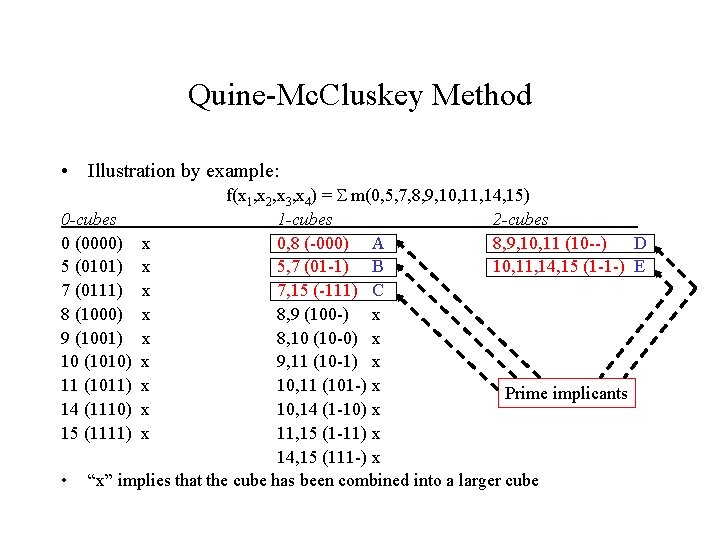
Quine-Mc. Cluskey Method • Illustration by example: f(x 1, x 2, x 3, x 4) = m(0, 5, 7, 8, 9, 10, 11, 14, 15) 0 -cubes 1 -cubes 2 -cubes 0 (0000) x 0, 8 (-000) A 8, 9, 10, 11 (10 --) D 5 (0101) x 5, 7 (01 -1) B 10, 11, 14, 15 (1 -1 -) E 7 (0111) x 7, 15 (-111) C 8 (1000) x 8, 9 (100 -) x 9 (1001) x 8, 10 (10 -0) x 10 (1010) x 9, 11 (10 -1) x 11 (1011) x 10, 11 (101 -) x Prime implicants 14 (1110) x 10, 14 (1 -10) x 15 (1111) x 11, 15 (1 -11) x 14, 15 (111 -) x • “x” implies that the cube has been combined into a larger cube

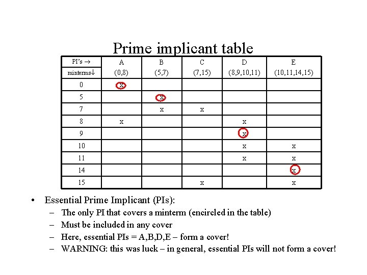
Prime implicant table PI’s minterms A (0, 8) 0 x B (5, 7) 5 x 7 x 8 C (7, 15) D (8, 9, 10, 11) E (10, 11, 14, 15) x x x 9 x 10 x x 11 x x 14 15 x x x • Essential Prime Implicant (PIs): – – The only PI that covers a minterm (encircled in the table) Must be included in any cover Here, essential PIs = A, B, D, E – form a cover! WARNING: this was luck – in general, essential PIs will not form a cover!

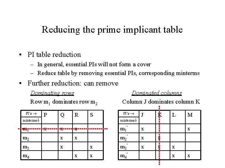
Reducing the prime implicant table • PI table reduction – In general, essential PIs will not form a cover – Reduce table by removing essential PIs, corresponding minterms • Further reduction: can remove Dominating rows Row m 1 dominates row m 2 PI’s P Q R S minterms m 1 Dominated columns Column J dominates column K PI’s J K M minterms x x m 1 ’ x m 2 x x m 2 ’ x x m 3 ’ x x x m 4 ’ m 4 L x x x

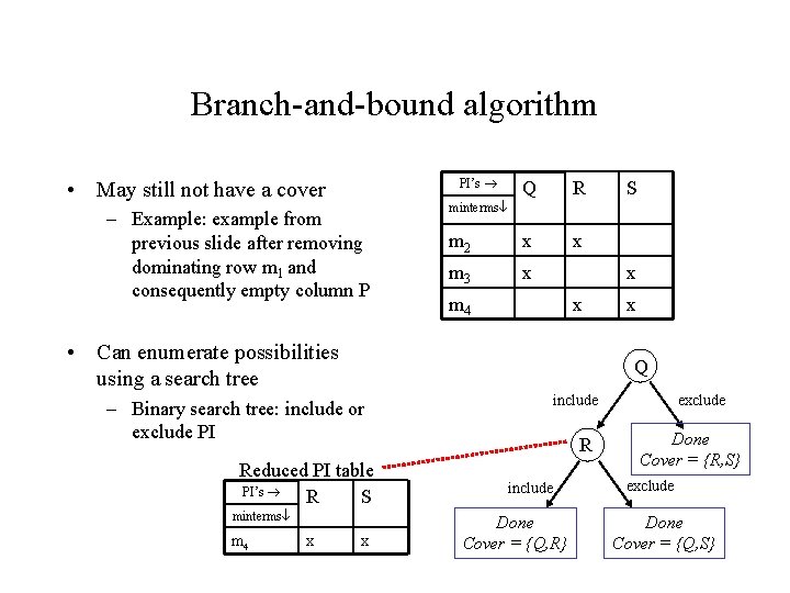
Branch-and-bound algorithm PI’s • May still not have a cover – Example: example from previous slide after removing dominating row m 1 and consequently empty column P Q R m 2 x x m 3 x minterms x m 4 x • Can enumerate possibilities using a search tree Reduced PI table PI’s R S minterms x x Q – Binary search tree: include or exclude PI m 4 S x include R include Done Cover = {Q, R} exclude Done Cover = {R, S} exclude Done Cover = {Q, S}

Branch-and-bound algorithm (contd. ) • ESPRESSO-EXACT – Implementation of branching algorithm from previous slide – Traversal to a leaf node of the tree yields a cover (though possibly not a minimum cost cover) – ESPRESSO-EXACT adds bounding at any node: • If Costnode + LBsubtree > Best_cost_so_far, do not search the subtree – Costnode = cost (e. g. , number of implicants) chosen so far – LBsubtree = a lower bound on the cost of a subtree (can be determined by solving a maximal independent set problem) – Best_cost_so_far = cost of best cover found so far through the traversal of the search tree; initialized to

Heuristic Logic Minimization • Apply a sequence of logic transformations to reduce a cost function • Transformations – Expand: • Input expansion – Enlarge cube by combining smaller cubes – Reduces total number of cubes • Output expansion – Use cube for one output to cover another – Reduce: break up cube into sub-cubes • Increases total number of cubes • Hope to allow overall cost reduction in a later expand operation – Irredundant • Remove redundant cubes from a cover

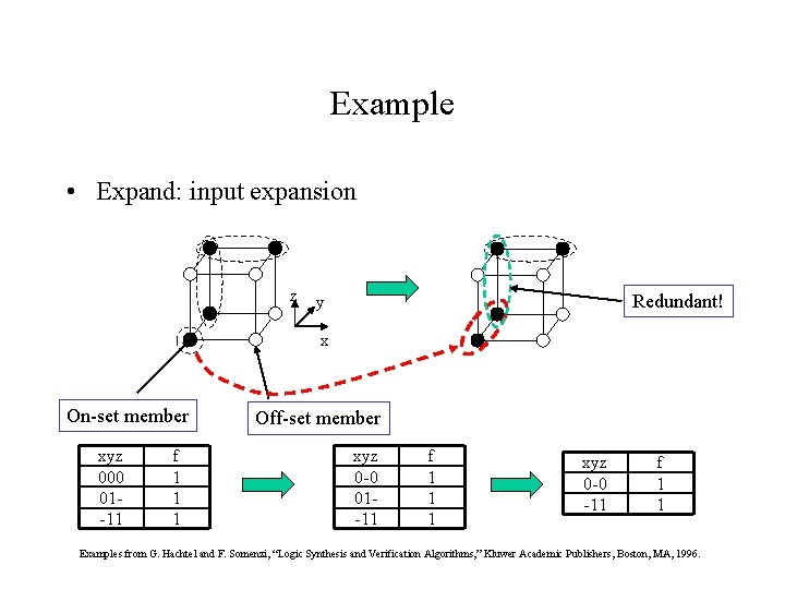
Example • Expand: input expansion z Redundant! y x On-set member xyz 000 01 -11 f 1 1 1 Off-set member xyz 0 -0 01 -11 f 1 1 1 xyz 0 -0 -11 f 1 1 Examples from G. Hachtel and F. Somenzi, “Logic Synthesis and Verification Algorithms, ” Kluwer Academic Publishers, Boston, MA, 1996.

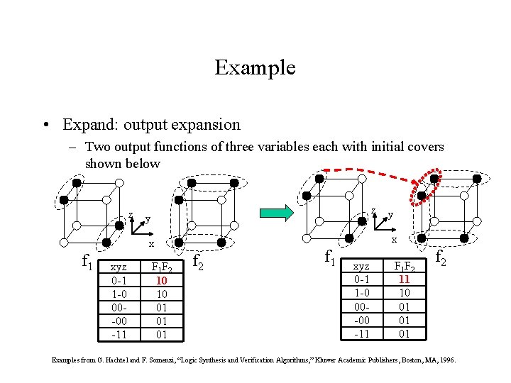
Example • Expand: output expansion – Two output functions of three variables each with initial covers shown below z z y x x f 1 xyz 0 -1 1 -0 00 -00 -11 F 1 F 2 10 10 01 01 01 y f 2 f 1 xyz 0 -1 1 -0 00 -00 -11 F 1 F 2 11 10 01 01 01 f 2 Examples from G. Hachtel and F. Somenzi, “Logic Synthesis and Verification Algorithms, ” Kluwer Academic Publishers, Boston, MA, 1996.

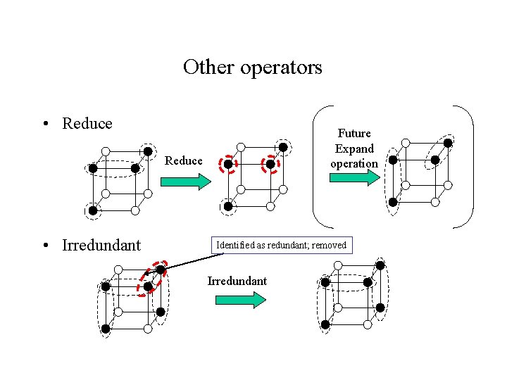
Other operators • Reduce Future Expand operation Reduce • Irredundant Identified as redundant; removed Irredundant

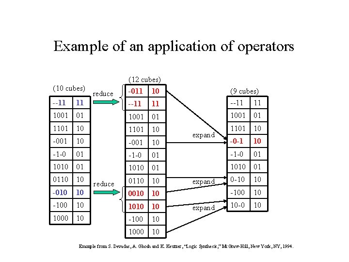
Example of an application of operators (10 cubes) (12 cubes) -011 10 --11 11 (9 cubes) --11 11 1001 01 1101 10 -001 10 -1 -0 01 -1 -0 1010 01 0110 10 -010 reduce expand 1101 10 -0 -1 10 01 -1 -0 01 1010 01 0110 10 10 0010 10 -100 10 10 1000 10 -100 10 1000 10 reduce expand 0 -10 10 -100 10 10 -0 10 Example from S. Devadas, A. Ghosh and K. Keutzer, “Logic Synthesis, ” Mc. Graw-Hill, New York, NY, 1994.

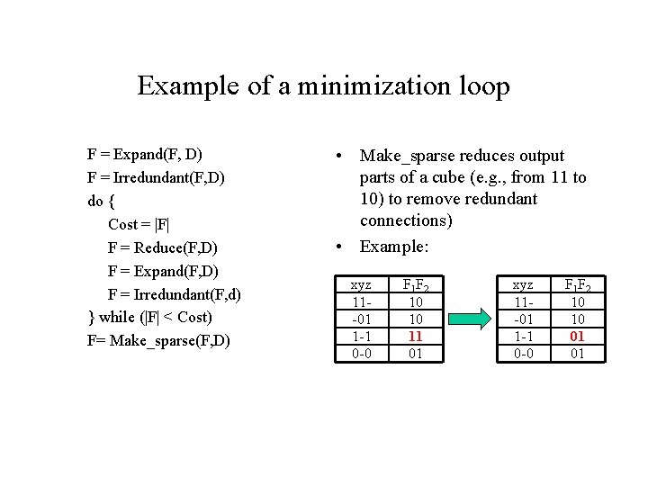
Example of a minimization loop F = Expand(F, D) F = Irredundant(F, D) do { Cost = |F| F = Reduce(F, D) F = Expand(F, D) F = Irredundant(F, d) } while (|F| < Cost) F= Make_sparse(F, D) • Make_sparse reduces output parts of a cube (e. g. , from 11 to 10) to remove redundant connections) • Example: xyz 11 -01 1 -1 0 -0 F 1 F 2 10 10 11 01 xyz 11 -01 1 -1 0 -0 F 1 F 2 10 10 01 01

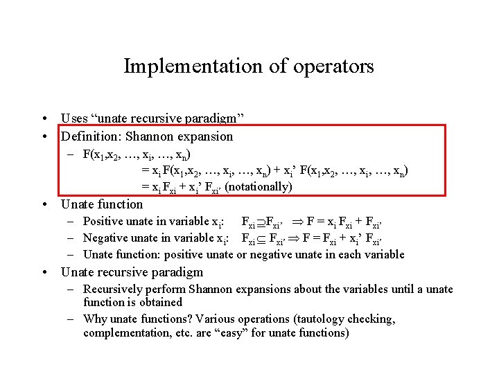
Implementation of operators • Uses “unate recursive paradigm” • Definition: Shannon expansion – F(x 1, x 2, …, xi, …, xn) = xi F(x 1, x 2, …, xi, …, xn) + xi’ F(x 1, x 2, …, xi, …, xn) = xi Fxi + xi’ Fxi’ (notationally) • Unate function – Positive unate in variable xi: Fxi’ F = xi Fxi + Fxi’ – Negative unate in variable xi: Fxi’ F = Fxi + xi’ Fxi’ – Unate function: positive unate or negative unate in each variable • Unate recursive paradigm – Recursively perform Shannon expansions about the variables until a unate function is obtained – Why unate functions? Various operations (tautology checking, complementation, etc. are “easy” for unate functions)

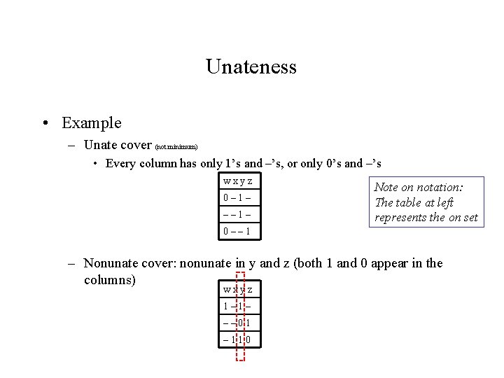
Unateness • Example – Unate cover (not minimum) • Every column has only 1’s and –’s, or only 0’s and –’s wxyz 0– 1– –– 1– Note on notation: The table at left represents the on set 0–– 1 – Nonunate cover: nonunate in y and z (both 1 and 0 appear in the columns) wxyz 1– 1– –– 01 – 110

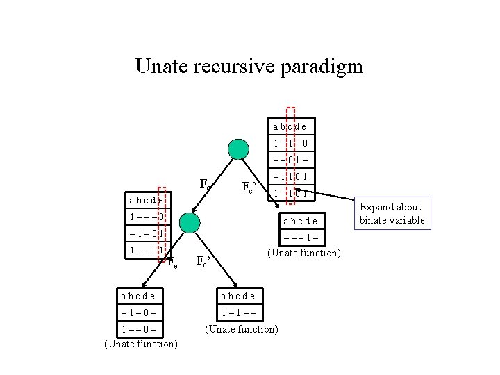
Unate recursive paradigm abcde 1– 1– 0 –– 01– Fc abcde Fc’ – 1101 1––– 0 abcde – 1– 01 ––– 1– 1–– 01 Fe (Unate function) Fe’ abcde – 1– 0– 1– 1–– 0– (Unate function) Expand about binate variable

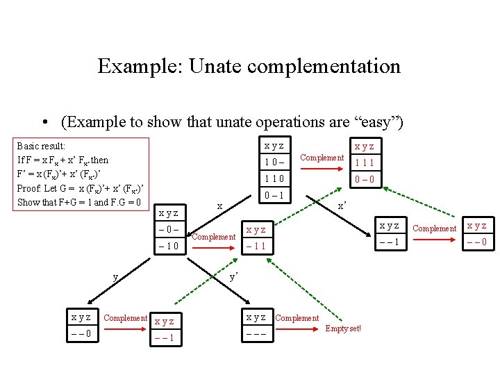
Example: Unate complementation • (Example to show that unate operations are “easy”) Basic result: If F = x Fx + x’ Fx’ then F’ = x (Fx)’+ x’ (Fx’)’ Proof: Let G = x (Fx)’+ x’ (Fx’)’ Show that F+G = 1 and F. G = 0 xyz 10– xyz Complement 110 xyz – 0– – 10 y 0– 1 x Complement 111 0– 0 x’ xyz – 11 –– 1 y’ xyz Complement x y z xyz –– 0 –– 1 ––– Complement Empty set! Complement xyz –– 0

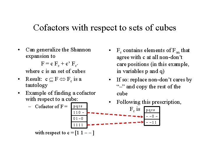
Cofactors with respect to sets of cubes • Can generalize the Shannon expansion to F = c Fc + c’ Fc’ where c is an set of cubes • Result: c F Fc is a tautology • Example of finding a cofactor with respect to a cube: – Cofactor of F = pqrs 110 – 01– 0 1111 with respect to c = [1 1 – – ] • Fc contains elements of Fon that agree with c at all non-don’t care positions (in this example, in variables p and q) • If so: replace non-don’t cares by “–” and copy the rest of the cube • Following this prescription, Fc is p q r s – – 0 – – – 11

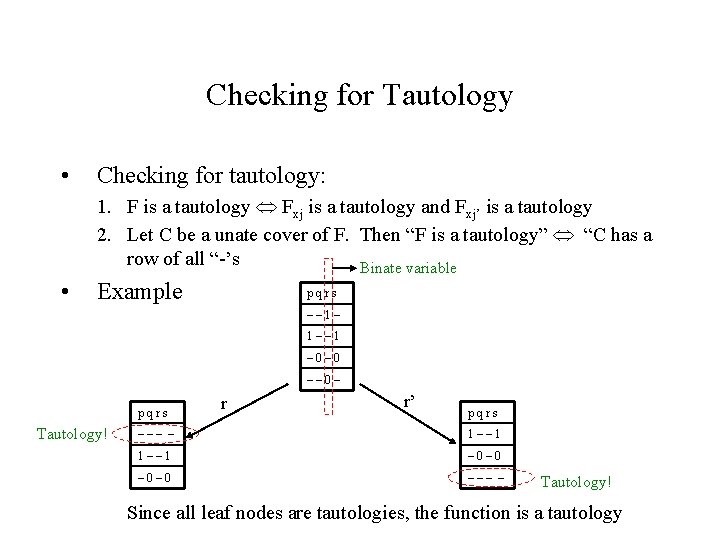
Checking for Tautology • Checking for tautology: 1. F is a tautology Fxj is a tautology and Fxj’ is a tautology 2. Let C be a unate cover of F. Then “F is a tautology” “C has a row of all “-’s Binate variable • Example pqrs –– 1– 1–– 1 – 0– 0 –– 0– pqrs Tautology! r r’ pqrs ––– – 1–– 1 – 0– 0 ––– – Tautology! Since all leaf nodes are tautologies, the function is a tautology

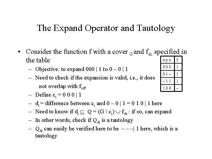
The Expand Operator and Tautology • Consider the function f with a cover G and fdc specified in xyz f the table 000 1 – Objective: to expand 000 | 1 to 0 – 0 | 1 01– 1 – Need to check if the expansion is valid, i. e. , it does – 1 1 1 not overlap with foff 100 – – Define ci = 0 0 0 | 1 – di = difference between ci and 0 – 0 | 1 = 0 1 0 | 1 here – Need to know if di Q = (G ci) fdc : if so, can expand – In other words, check if Qdi is a tautology – Qdi can easily be verified here to be – – –| 1 here, which is a tautology

The Irredundant Operator and Tautology • Objective: to check if a cube ci in a cover G of function F is redundant – In other words, check if ci Q = (G ci) Fdc – In other words, check if Qci is a tautology

Multilevel logic optimization • Motivation – Two-level optimization (SOP, POS) is too limiting – Useful for structures like PLA’s, but most circuits are not designed in that way – May require gates with a large number of inputs – Restricts “sharing” of logic gates between outputs – Multilevel optimization permits more than two levels of gates between the inputs and the outputs – Necessarily heuristic Reference for this part: G. De Micheli, “Synthesis and Optimization of Digital Circuits, ” Mc. Graw-Hill, New York, NY, 1994.

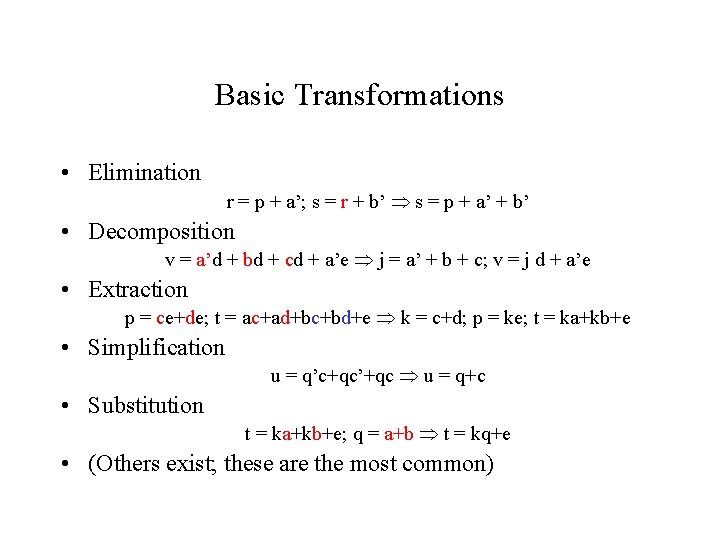
Basic Transformations • Elimination r = p + a’; s = r + b’ s = p + a’ + b’ • Decomposition v = a’d + bd + cd + a’e j = a’ + b + c; v = j d + a’e • Extraction p = ce+de; t = ac+ad+bc+bd+e k = c+d; p = ke; t = ka+kb+e • Simplification u = q’c+qc’+qc u = q+c • Substitution t = ka+kb+e; q = a+b t = kq+e • (Others exist; these are the most common)

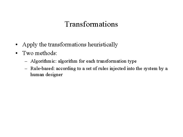
Transformations • Apply the transformations heuristically • Two methods: – Algorithmic: algorithm for each transformation type – Rule-based: according to a set of rules injected into the system by a human designer

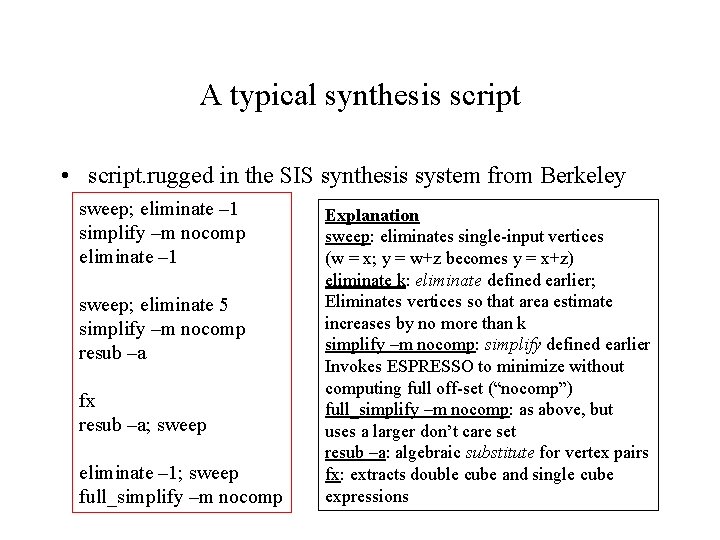
A typical synthesis script • script. rugged in the SIS synthesis system from Berkeley sweep; eliminate – 1 simplify –m nocomp eliminate – 1 sweep; eliminate 5 simplify –m nocomp resub –a fx resub –a; sweep eliminate – 1; sweep full_simplify –m nocomp Explanation sweep: eliminates single-input vertices (w = x; y = w+z becomes y = x+z) eliminate k: eliminate defined earlier; Eliminates vertices so that area estimate increases by no more than k simplify –m nocomp: simplify defined earlier Invokes ESPRESSO to minimize without computing full off-set (“nocomp”) full_simplify –m nocomp: as above, but uses a larger don’t care set resub –a: algebraic substitute for vertex pairs fx: extracts double cube and single cube expressions

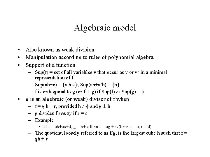
Algebraic model • Also known as weak division • Manipulation according to rules of polynomial algebra • Support of a function – Sup(f) = set of all variables v that occur as v or v’ in a minimal representation of f – Sup(ab+c) = {a, b, c}; Sup(ab+a’b) = {b} – f is orthogonal to g (or f g) if Sup(f) Sup(g) = • g is an algebraic (or weak) divisor of f when – f = g h + r, provided h and g h – g divides f evenly if r = – Example • If f = ab+ac+d; g = b+c, then f = ag + d (here h = a, r = d) – The quotient, loosely referred to as f/g, is the largest cube h such that f = gh + r

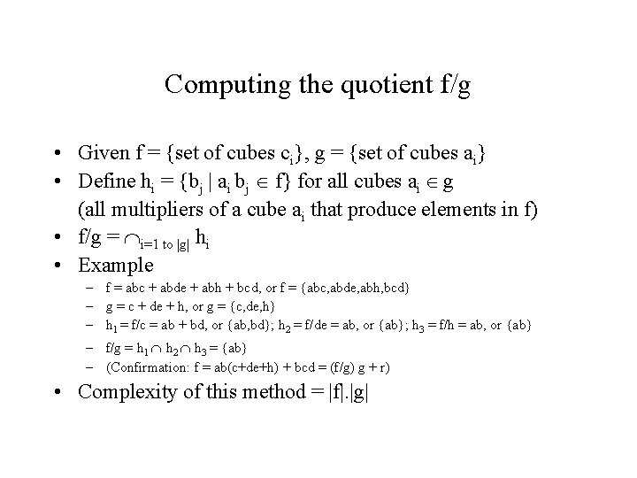
Computing the quotient f/g • Given f = {set of cubes ci}, g = {set of cubes ai} • Define hi = {bj | ai bj f} for all cubes ai g (all multipliers of a cube ai that produce elements in f) • f/g = i=1 to |g| hi • Example – f = abc + abde + abh + bcd, or f = {abc, abde, abh, bcd} – g = c + de + h, or g = {c, de, h} – h 1 = f/c = ab + bd, or {ab, bd}; h 2 = f/de = ab, or {ab}; h 3 = f/h = ab, or {ab} – f/g = h 1 h 2 h 3 = {ab} – (Confirmation: f = ab(c+de+h) + bcd = (f/g) g + r) • Complexity of this method = |f|. |g|

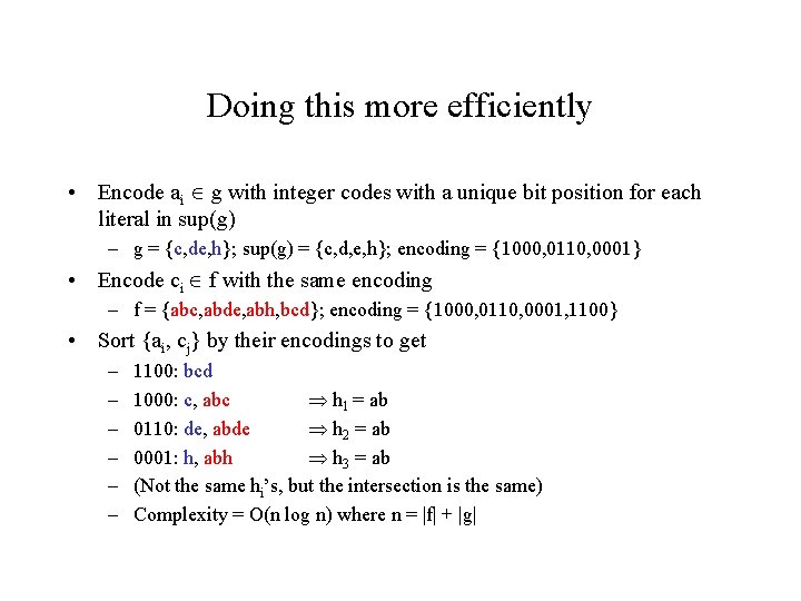
Doing this more efficiently • Encode ai g with integer codes with a unique bit position for each literal in sup(g) – g = {c, de, h}; sup(g) = {c, d, e, h}; encoding = {1000, 0110, 0001} • Encode ci f with the same encoding – f = {abc, abde, abh, bcd}; encoding = {1000, 0110, 0001, 1100} • Sort {ai, cj} by their encodings to get – – – 1100: bcd 1000: c, abc h 1 = ab 0110: de, abde h 2 = ab 0001: h, abh h 3 = ab (Not the same hi’s, but the intersection is the same) Complexity = O(n log n) where n = |f| + |g|

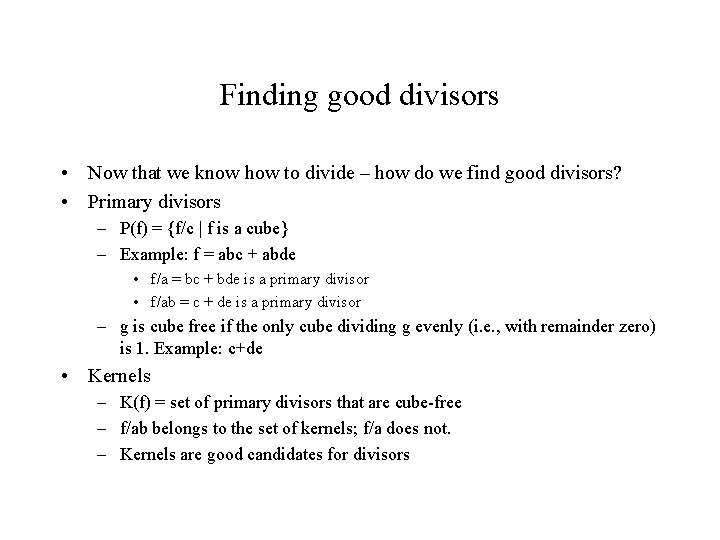
Finding good divisors • Now that we know how to divide – how do we find good divisors? • Primary divisors – P(f) = {f/c | f is a cube} – Example: f = abc + abde • f/a = bc + bde is a primary divisor • f/ab = c + de is a primary divisor – g is cube free if the only cube dividing g evenly (i. e. , with remainder zero) is 1. Example: c+de • Kernels – K(f) = set of primary divisors that are cube-free – f/ab belongs to the set of kernels; f/a does not. – Kernels are good candidates for divisors

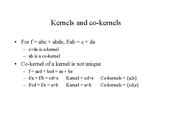
Kernels and co-kernels • For f = abc + abde, f/ab = c + de – c+de is a kernel – ab is a co-kernel • Co-kernel of a kernel is not unique – f = acd + bcd + ae + be – f/a = f/b = cd+e Kernel = cd+e – f/cd = f/e = a+b Kernel = a+b Co-kernels = {a, b} Co-kernels = {cd, e}

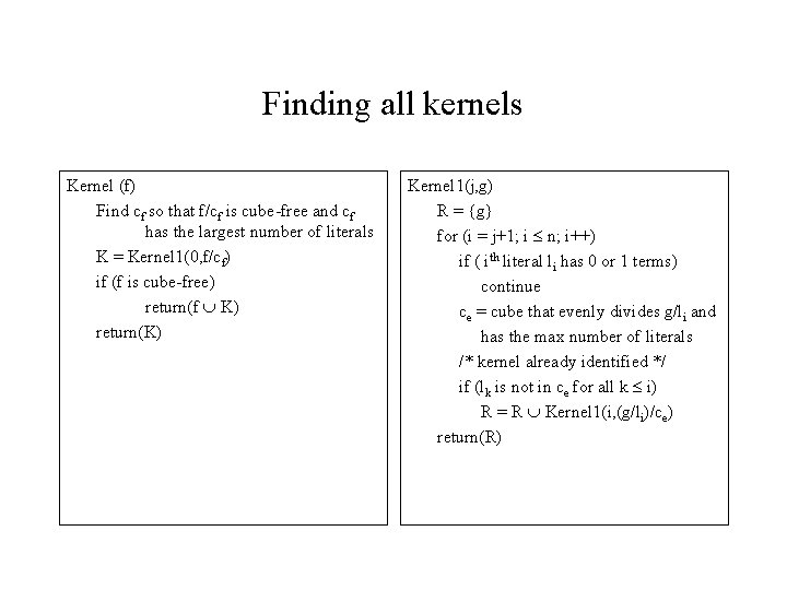
Finding all kernels Kernel (f) Find cf so that f/cf is cube-free and cf has the largest number of literals K = Kernel 1(0, f/cf) if (f is cube-free) return(f K) return(K) Kernel 1(j, g) R = {g} for (i = j+1; i n; i++) if ( ith literal li has 0 or 1 terms) continue ce = cube that evenly divides g/li and has the max number of literals /* kernel already identified */ if (lk is not in ce for all k i) R = R Kernel 1(i, (g/li)/ce) return(R)

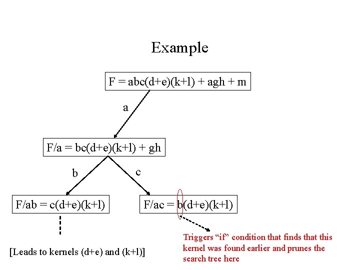
Example F = abc(d+e)(k+l) + agh + m a F/a = bc(d+e)(k+l) + gh b F/ab = c(d+e)(k+l) c F/ac = b(d+e)(k+l) [Leads to kernels (d+e) and (k+l)] Triggers “if” condition that finds that this kernel was found earlier and prunes the search tree here

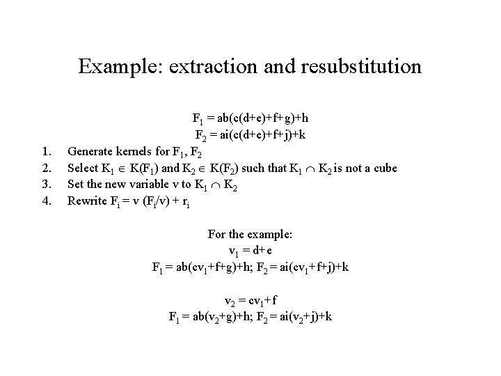
Example: extraction and resubstitution 1. 2. 3. 4. F 1 = ab(c(d+e)+f+g)+h F 2 = ai(c(d+e)+f+j)+k Generate kernels for F 1, F 2 Select K 1 K(F 1) and K 2 K(F 2) such that K 1 K 2 is not a cube Set the new variable v to K 1 K 2 Rewrite Fi = v (Fi/v) + ri For the example: v 1 = d+e F 1 = ab(cv 1+f+g)+h; F 2 = ai(cv 1+f+j)+k v 2 = cv 1+f F 1 = ab(v 2+g)+h; F 2 = ai(v 2+j)+k

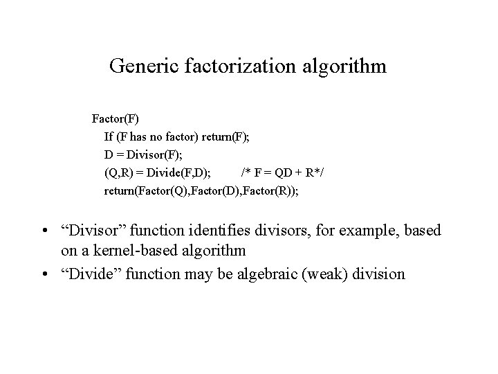
Generic factorization algorithm Factor(F) If (F has no factor) return(F); D = Divisor(F); (Q, R) = Divide(F, D); /* F = QD + R*/ return(Factor(Q), Factor(D), Factor(R)); • “Divisor” function identifies divisors, for example, based on a kernel-based algorithm • “Divide” function may be algebraic (weak) division

Don’t care based optimization: an outline • Two types of don’t cares considered here – Satisfiability don’t cares – Observability don’t cares – Others: SPFD’s (sets of pairs of functions to be differentiated) • Satisfiability don’t cares (SDC’s) – Example: Consider • Y 1 = a’b’ Y 2 = c’d’ Y 3 = Y 1’Y 2’ • Since Y 1 = a’b’ is enforced by one equation, the minterms of “Y 1 (a’b’)” can be considered to be don’t cares • In other words, Y 1 a’b’ + Y 1(a+b) corresponds to a don’t care • Similarly, “Y 2 (c’d’)” is also a don’t care

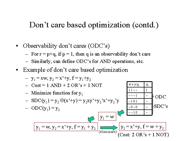
Don’t care based optimization (contd. ) • Observability don’t cares (ODC’s) – For r = p+q, if p = 1, then q is an observability don’t care – Similarly, can define ODC’s for AND operations, etc. • Example of don’t care based optimization – – – y 1 = xw, y 2 = x’+y, f = y 1+y 2 Cost = 1 AND + 2 OR’s + 1 NOT Minimize function for y 1 SDC(y 1) = y 2 (x’+y) = y 2 xy’+y 2’x’+y 2’y ODC(y 1) = y 2 y 1 = w, y 2 = x’+y, f = y 1 + y 2 (eliminate) w x y y 2 y 1 11–– 1 – – 101 – – 0– 0 – –– 10 – ODC SDC’s y 2 = x’+y, f = w + y 2 (Cost: 2 OR’s + 1 NOT)

Acknowledgements • Hardly anything in these notes is original, and they borrow heavily from sources such as – G. De Micheli, “Synthesis and Optimization of Digital Circuits, ” Mc. Graw -Hill, New York, NY, 1994. – S. Devadas, A. Ghosh and K. Keutzer, “Logic Synthesis, ” Mc. Graw-Hill, New York, NY, 1994 – G. Hachtel and F. Somenzi, “Logic Synthesis and Verification Algorithms, ” Kluwer Academic Publishers, Boston, MA, 1996. – Notes from Prof. Brayton's synthesis class at UC Berkeley (http: //wwwcad. eecs. berkeley. edu/~brayton/courses/219 b. html) – Notes from Prof. Devadas's CAD class at MIT (http: //glenfiddich. lcs. mit. edu/~devadas/6. 373/lectures) – Possibly other sources that I may have omitted to acknowledge (my apologies)