Logic Synthesis Equivalence Checking Courtesy RK Brayton UCB

Logic Synthesis Equivalence Checking Courtesy RK Brayton (UCB) and A Kuehlmann (Cadence) 1

Application of EC in m. P Designs Architectural Specification (informal) Cycle Simulation Test Programs RTL Specification (Verilog, VHDL) Circuit Implementation (Schematic) Equivalence Checking Circuit Simulation Layout Implementation (GDS II) 2

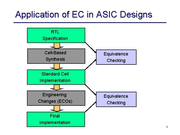
Application of EC in ASIC Designs RTL Specification Cell-Based Synthesis Equivalence Checking Standard Cell Implementation Engineering Changes (ECOs) Equivalence Checking Final Implementation 3

Basic Model Finite State Machines X=(x 1, x 2, …, xn) l S=(s 1, s 2, …, sn) d Y=(y 1, y 2, …, yn) S’=(s’ 1, s’ 2, …, s’n) M(X, Y, S, S 0, d, l): X: Inputs Y: Outputs S: Current State S 0: Initial State(s) d: X ´ S ® S (next state function) l: X ´ S ® Y (output function) D Delay element: • Clocked: synchronous • single-phase clock, multiple-phase clocks • Unclocked: asynchronous 4

Finite State Machines Equivalence Build Product Machine M 1´ M 2: l d y 1 {0, 0, . . . , 0} {X 1, X 2, …, Xn} D M 1 l d D y 2 M 2 Definition: M 1 and M 2 are functionally equivalent iff the product machine M 1 ´ M 2 produces a constant 0 for all valid input sequences {X 1, …, Xn}. 5

General Approach to EC State Space of S = M 1 ´ M 2 miscomparing states i. e. l ¹ 0 comparing states i. e. l = 0 Initial State S 0 R “Good half” r(s) = 1 (S-R) “Bad half” r(s) = Inductive proof of equivalence: Find subset R Í S with characteristic function f: S® {0, 1} such that: 1. r(s 0) = 1 (initial state is in good half) 2. (r(s) = 1) Þ r(d(x, s)) = 1 (all states from good half lead go to states in good half) 3. (r(s) = 1) Þ l(x, s)) = 1 (all states in good half are comparing states) 6

Proving R 1. Use SAT check to verify that initial state S 0 is contained in R: (r(s 0) = 1) 2. Use SAT check to verify that: • states in R are comparing states • all states from R lead only to states in R x s 0? F r 0? D r 7

Soundness and Completeness • With a candidate for R we can: – prove equivalance • that means the method is “sound” • we will not produce “false positives” – but not disprove it: • that means the method is “incomplete” • we may produce “false negatives” 8

How Do We Obtain R? • Reachability analysis: – state traversal until no more states can be explored • forward • backward • explicit • symbolic • Relying on the design methodology to provide R: – equivalent state encoding in both machines – synthesis tool provides hint for R from sequential optimization • manual register correspondence • automatic register correspondence • Combination of them 9

Combinational EC • Industrial EC checkers almost exclusively use an combinational EC paradigm – sequential EC is too complex, can only be applied to design with a few hundred state bits – combinational methods scale linearly with the design size for a given fixed size and “functional complexity” of the individual cones • Still, pure BDDs are plain SAT solver cannot handle all cones – BDDs can be built for about 80% of the cones of high-speed designs – less for complex ASICs – plain SAT blows up on a “Miter” structure • Contemporary method highly exploit structural similarity of designs to be compared 10

Miter Structure for Combinational EC x 0? Basic methods: • random simulation, good for finding miscompares • BDD based and modifications • structural SAT based with modifications 11

History of Equivalence Checking • • • SAS (IBM 1978 - 1994): – standard equivalence checking tool running on mainframes – based on the DBA algorithm (“BDDs in time”) – verified manual cell-based designs against RTL spec – handling of entire processor designs • application of “proper cutpoints” • application of synthesis routines to make circuits structurally similar • special hacks for hard problems BEC (IBM 1991 - 1996): – workstation based re-implementation of SAS – mainly used in Boole. Dozer synthesis environment Verity (IBM 1992 - today): – originally developed for switch-level designs – today IBMs standard EC tool for any combination of switch-, gate-, and RTL designs 12

History of Equivalence Checking • Chrysalis (1994 - now Avanti): – based on ATPG technology and cutpoint exploitation – very weak if many cutpoints present – did not adopt BDDs for a long time • Formality (1997 - Synopsys) – multi-engine technology including strong structural matching techniques • Verplex (1998) – strong multi-engine based tool – to our knowledge heavy SAT-based – very fast front-end 13

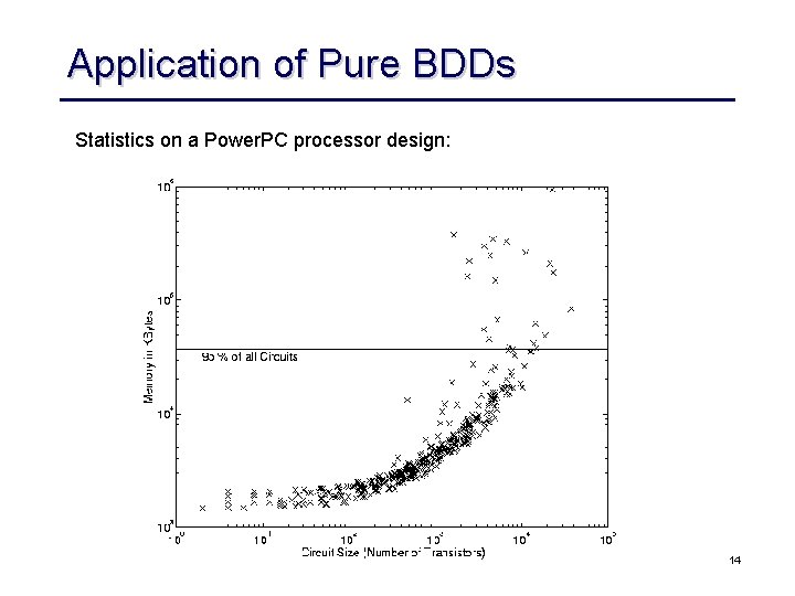
Application of Pure BDDs Statistics on a Power. PC processor design: 14

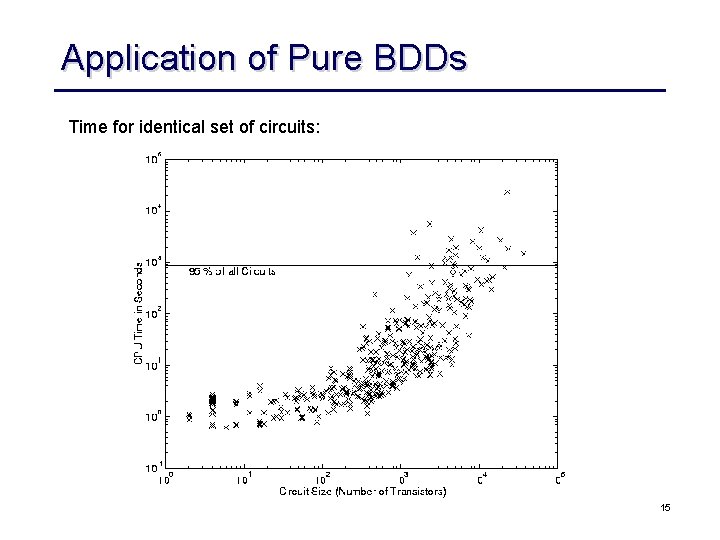
Application of Pure BDDs Time for identical set of circuits: 15

Functional Equivalent Nets (%) Structural Similarity Circuit Size 16

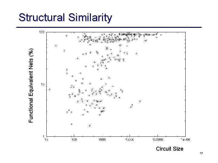
Functional Equivalent Nets (%) Structural Similarity Circuit Size 17

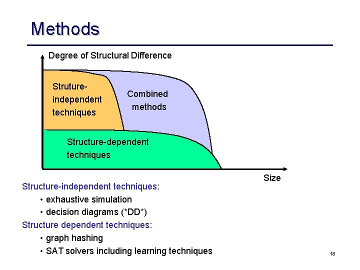
Methods Degree of Structural Difference Strutureindependent techniques Combined methods Structure-dependent techniques Structure-independent techniques: • exhaustive simulation • decision diagrams (*DD*) Structure dependent techniques: • graph hashing • SAT solvers including learning techniques Size 18

Handling Constraints Input constraints: • non-occuring input values (don’t cares) • non-reachable states • candidate for R 1. Input Mapping: x MAP 0? x’ 2. Output Masking: x Characteristic function for constraint 0? c 19

Cutpoint-based EC Cutpoints are used to partition the Miter v 1 f 2 f 3 v 2 0? x 0? v 1 f 2 f 3 v 2 Cutpoint guessing: • Compute net signature with random simulator • Sort signatures + select cutpoints • Iteratively verify and refine cutpoints • Verify outputs 20

False Negatives Outputs may miscompare for invalid cutpoint values: vz x y z v out vz v xy 00 10 11 01 00 01 11 1 1 10 1 1 xy 1 1 00 10 11 01 00 01 11 10 Constraint: c = (v º y+z) 1 1 1 vz xy 00 00 10 11 01 11 1 1 10 1 1 What can we do about false negatives: • constrain input space to c = (v º y+z) • if (v in SUPPORT(out) then out = compose(out, v, fv) 21

Permissible Cutpoints Testable for s-a-0 or s-a-1? Based in ATPG: - test for s-a-0 at output checks for permissible functions x - test for s-a-1 output checks for inverse permissibe functions Permissible functions: - successively merge circuits from input to outputs x 0? 22

Sequential Equivalence Checking • If combinational verification paradigm fails (e. g. we have no name matching • Two options: – run full sequential verification based on state traversal • very expensive but most general – try to match registers automatically • functional register correspondence • structural register correspondence 23

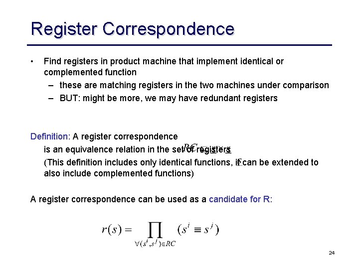
Register Correspondence • Find registers in product machine that implement identical or complemented function – these are matching registers in the two machines under comparison – BUT: might be more, we may have redundant registers Definition: A register correspondence is an equivalence relation in the set of registers (This definition includes only identical functions, it can be extended to also include complemented functions) A register correspondence can be used as a candidate for R: 24

Functional Register Correspondence Algorithm REGISTER_CORRESPONDENCE { RC’ = {(si, sj) | si 0 = sj 0} // start with registers with do { // identical initial states RC = RC’ r(s) = P" (si, sj) ÎRC (si º sj) RC’ = {(si, sj) | (si, sj) Î RC Ù di(x, s)=dj(x, s) Ù r(s)} } while (RC’ != RC) return RC } In essence: • the algorithm starts with an initial partitioning with two equivalence classes, one for each initial value • the algorithm computes iteratively the next state function, assuming that the RC is correct - if yes, fixed point is reached and RC returned - if no, split equivalence classes along the miscompares 25

Example x s 1 Instead of using constraint, use fresh variable for each class s 2 1 1 s 1=1 s 2=1 s 3=1 s 4=1 s 5=1 v s 3 1 s 1= x Å v s 4= x Å v v 1 s 4 s 5 1 1 Result: {s 1, s 4} {s 2, s 3, s 5} s 2= Øv s 3= Øv s 5= Øv v 2 s 1= x Å v 1 s 4= x Å v 1 s 2= Ø(v 1 v 2) v 1 s 5= Ø(v 1 v 2) s 3= Ø(v 1 v 2) v 2 26

Problems with Functional Reg. Corr. • In case of micomparing designs – effect of miscomparing cone may ripple through entire algorithm and split all equivalence classes until they contain only single registers – difficult to debug since no hint of error location • Solution: – relaxation of equivalence criteria • e. g. structural register correspondence algorithm based on support set of registers • combined techniques with name mapping, functional/structural criteria 27

Sequential Equivalence Checking • In case that combinational equivalence checking model fails: – use generalized register correspondence to also consider retiming • in essence, use all internal nets as candidates for possible matches • Worst case: full sequential verification – Prove that the output of the product machine is not satisfiable (sequentially) – special case of general property checking 28

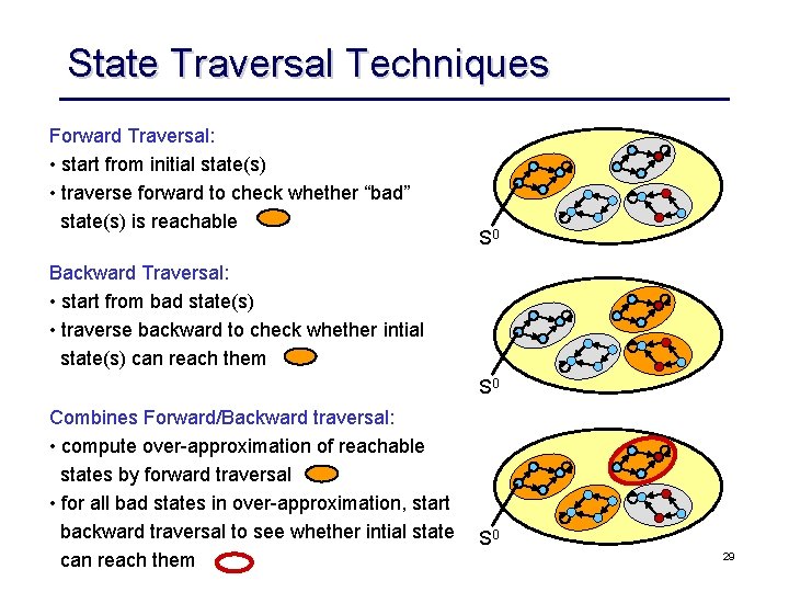
State Traversal Techniques Forward Traversal: • start from initial state(s) • traverse forward to check whether “bad” state(s) is reachable S 0 Backward Traversal: • start from bad state(s) • traverse backward to check whether intial state(s) can reach them S 0 Combines Forward/Backward traversal: • compute over-approximation of reachable states by forward traversal • for all bad states in over-approximation, start backward traversal to see whether intial state can reach them S 0 29

Transition Relation t(s, s’): X=0 Examples: 0 1 X=1 1 30

Image and Pre-Image of States Image of a set of states r(s): Example: 0 2 Pre-Image of a set of states r(s): r(s) = (s º 0) Ú (s º 1) {0, 1} t(s, s’) = (s º 0) Ù (s’ º 2) Ú (s º 0) Ù (s’ º 3) Ú (s º 1) Ù (s’ º 3) Ú (s º 2) Ù (s’ º 4) {(0, 2), (0, 3), (1, 3), (2, 4)} tÙr = (s º 0) Ù (s’ º 2) Ú (s º 0) Ù (s’ º 3) Ú (s º 1) Ù (s’ º 3) {(0, 2), (0, 3), (1, 3)} 4 1 r(s) 3 Img(t, r(s)) $s. (r Ù t) = (s º 2) Ú (s’ º 3) {(2, 3)} 31

Forward State Traversal Algorithm TRAVERSE_FORWARD(t, l , S 0) { reached = Æ current = S 0 // start from init while (reached ¹ (reached Ú current)) { // fixed point reached = reached Ú current // add new states next = IMG(t, current) // one trans. current = next // rename variab. } return $x. (l(x, s) Ù reached) } Example: 0 1 3 2 4 5 6 Iteration: Reached: Current: Next: 1 {0} {1, 2} 2 {0, 1, 2} {1, 2, 3} 3 {0, 1, 2, 3} 32

Backward State Traversal Algorithm TRAVERSE_BACKWARD(t, l , S 0) { reached = Æ current = $x. (l(x, s)=1) // start from bad while (reached ¹ (reached Ú current)) { // fixed point reached = reached Ú current // add new states previous = PRE_IMG(t, current) // one trans. current = previous // rename variab. } return (S 0 Ù reached) } Example: 0 1 3 2 4 5 6 Iteration: Reached: Current: Previous: 1 {6} {4} 2 {4, 6} {4, 5} 3 {4, 5, 6} 33