Logic Programming Part 2 Lists Backtracking Optimization via

Logic Programming – Part 2 • • • Lists Backtracking Optimization (via the cut operator) Meta-Circular Interpreters

Lists – Basic Examples �[] – The empty list �[X, 2, f(Y)] – A 3 element list �[X|Xs] – A list starting with X. Xs is a list as well. �Example [3|5|[]] - [3, 5] may be written as

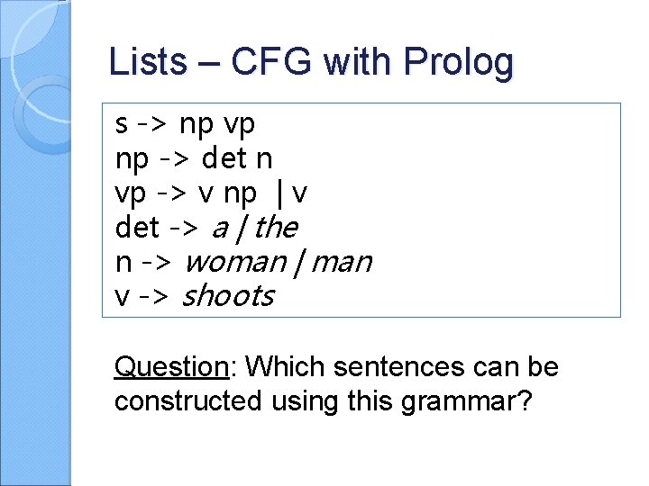
Lists – CFG with Prolog s -> np vp np -> det n vp -> v np | v det -> a | the n -> woman | man v -> shoots Question: Which sentences can be constructed using this grammar?

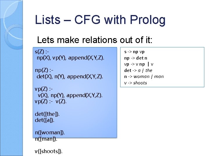
Lists – CFG with Prolog Lets make relations out of it: s(Z) : np(X), vp(Y), append(X, Y, Z). np(Z) : det(X), n(Y), append(X, Y, Z). vp(Z) : v(X), np(Y), append(X, Y, Z). vp(Z) : - v(Z). det([the]). det([a]). n([woman]). n([man]). v([shoots]). s -> np vp np -> det n vp -> v np | v det -> a | the n -> woman | man v -> shoots

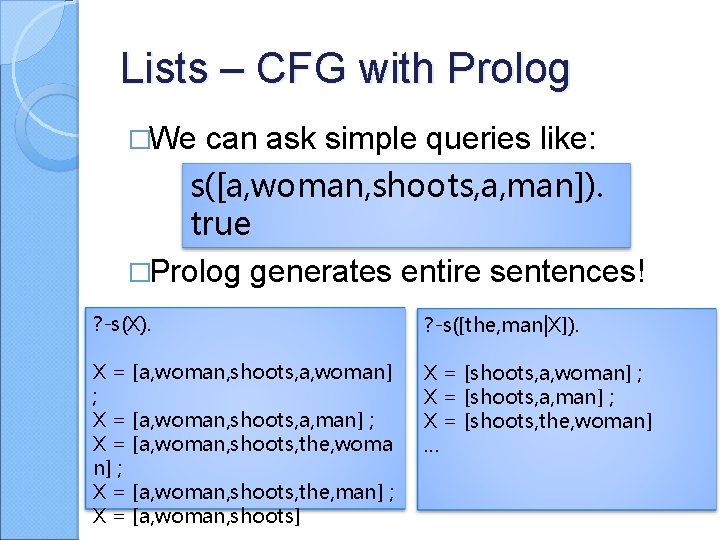
Lists – CFG with Prolog �We can ask simple queries like: s([a, woman, shoots, a, man]). true �Prolog generates entire sentences! ? -s(X). ? -s([the, man|X]). X = [a, woman, shoots, a, woman] ; X = [a, woman, shoots, a, man] ; X = [a, woman, shoots, the, woma n] ; X = [a, woman, shoots, the, man] ; X = [a, woman, shoots] X = [shoots, a, woman] ; X = [shoots, a, man] ; X = [shoots, the, woman] …

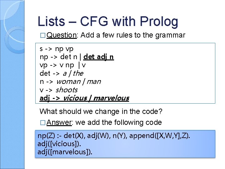
Lists – CFG with Prolog � Question: Add a few rules to the grammar s -> np vp np -> det n | det adj n vp -> v np | v det -> a | the n -> woman | man v -> shoots adj -> vicious | marvelous What should we change in the code? � Answer: we add the following code np(Z) : - det(X), adj(W), n(Y), append([X, W, Y], Z). adj([vicious]). adj([marvelous]).

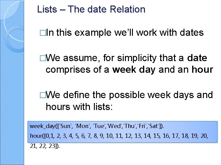
Lists – The date Relation �In this example we’ll work with dates �We assume, for simplicity that a date comprises of a week day and an hour �We define the possible week days and hours with lists: week_day(['Sun', 'Mon', 'Tue', 'Wed', 'Thu', 'Fri', 'Sat']). hour([0, 1, 2, 3, 4, 5, 6, 7, 8, 9, 10, 11, 12, 13, 14, 15, 16, 17, 18, 19, 20, 21, 22, 23]).

Lists – The date Relation �Q: How can we tell if hour 2 is before 9? �A: 1. A < relation isn’t really possible to implement. (More details in the PS document) 2. We can only do so by checking precedence in the lists above. week_day(['Sun', 'Mon', 'Tue', 'Wed', 'Thu', 'Fri', 'Sat']). hour([0, 1, 2, 3, 4, 5, 6, 7, 8, 9, 10, 11, 12, 13, 14, 15, 16, 17, 18, 19, 20, 21, 22, 23]).

Lists – The date Relation date([H, W]) : - hour(Hour_list), member(H, Hour_list), week_day(Weekday_list), member(W, Weekday_list). date. LT( date([_, W 1]), date([_, W 2]) ) : week_day(Weekday_list), precedes(W 1, W 2, Weekday_list). date. LT( date([H 1, W]), date([H 2, W]) ) : hour(Hour_list), precedes(H 1, H 2, Hour_list). Example queries: ? - date([1, 'Sun']). true date. LT(date([5, 'Mon']), date([1, 'Tue'])). true

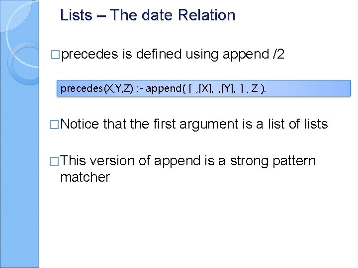
Lists – The date Relation �precedes is defined using append /2 precedes(X, Y, Z) : - append( [_, [X], _, [Y], _] , Z ). �Notice �This that the first argument is a list of lists version of append is a strong pattern matcher

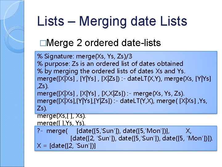
Lists – Merging date Lists �Merge 2 ordered date-lists % Signature: merge(Xs, Ys, Zs)/3 % purpose: Zs is an ordered list of dates obtained % by merging the ordered lists of dates Xs and Ys. merge([X|Xs] , [Y|Ys] , [X|Zs]) : - date. LT(X, Y), merge(Xs, [Y|Ys] , Zs). merge([X|Xs] , [X|Ys] , [X, X|Zs]) : - merge(Xs, Ys, Zs). merge([X|Xs], [Y|Ys], [Y|Zs]) : - date. LT(Y, X), merge( [X|Xs] , Ys, Zs). merge(Xs, [ ], Xs). merge([ ], Ys). ? - merge( [date([5, 'Sun']), date([5, 'Mon'])], X, [date([2, 'Sun']), date([5, 'Mon'])]). X = [date([2, 'Sun'])]

merge([d 1, d 3, d 5], [d 2, d 3], Xs) {X_1=d 1, Xs_1=[d 3, d 5], Y_1=d 2, Ys_1=[d 3], Xs=[d 1|Zs_1] } Rule 1 Rule 3 – failure branch… date. LT(d 1, d 2), merge([d 3, d 5], [d 2, d 3] , Zs_1) Rule 2 – failure branch… merge([d 3, d 5], [d 2, d 3] , Zs_1) Rule 1 – failure branch… Rule 2 – failure branch… { X_2=d 3, Xs_2=[d 5], Y_2=d 2, Ys_2=[d 3], Zs_1=[d 2|Zs_2]} Rule 3 date. LT(d 2, d 3), merge([d 3, d 5], [d 3] , Zs_2) Rule 3 – failure branch… Rule 1 – failure branch… { X_3=d 3, Xs_3=[d 5], Ys_3=[], Zs_2=[d 3, d 3|Zs_3] } Rule 2 merge([d 5], [] , Zs_3) { Xs_4=[d 5], Zs_3=[d 5] } Fact 4 true

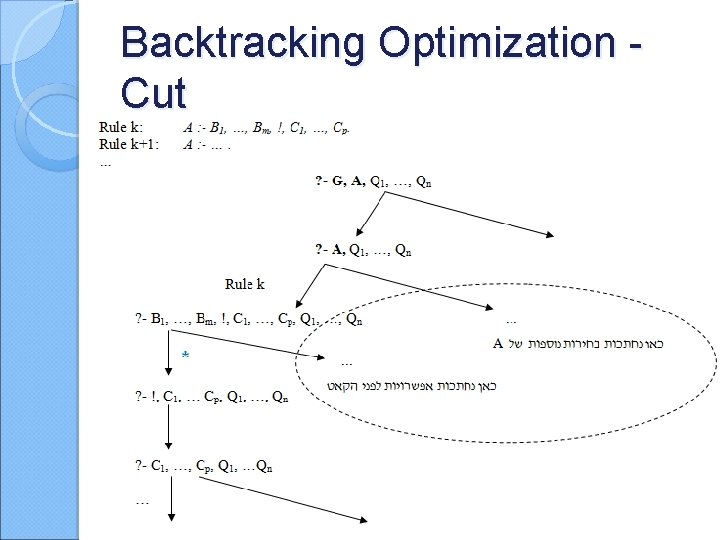
Backtracking Optimization Cut The cut operator (denoted ‘!’) allows to prune trees from unwanted branches. �A cut prunes all the goals below it �A cut prunes all alternative solutions of goals to the left of it �A cut does not affect the goals to it’s right �The cut operator is a goal that always

Backtracking Optimization Cut

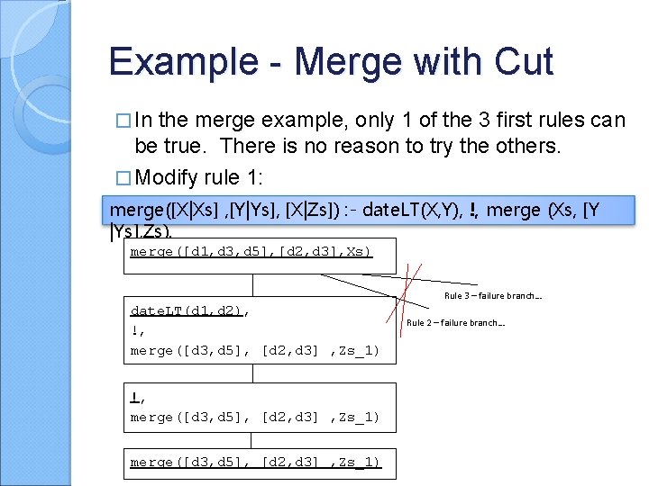
Example - Merge with Cut � In the merge example, only 1 of the 3 first rules can be true. There is no reason to try the others. � Modify rule 1: merge([X|Xs] , [Y|Ys], [X|Zs]) : - date. LT(X, Y), !, merge (Xs, [Y |Ys], Zs). merge([d 1, d 3, d 5], [d 2, d 3], Xs) Rule 3 – failure branch… date. LT(d 1, d 2), !, merge([d 3, d 5], [d 2, d 3] , Zs_1) Rule 2 – failure branch…

Another Example �How many results does this query ? - return? merge([], X). X = []; No �Why does this happen? The query fits both rules 4 and 5 �How can we avoid this? merge(Xs, : - !. 4 Add cut [to], Xs) rule

Meta-Circular Interpreter Version 1 % Signature: solve(Goal)/1 % Purpose: Goal is true if it is true when posed to the original program P. solve(true) : - !. solve( (A, B) ) : - solve(A), solve(B). solve(A) : - clause(A, B), solve(B). clause finds the first rule unifying with A with body B ? - clause( parent(X, isaac), Body). X = abraham Body = true ? - clause(ancestor(abraham, P), Body). P = Y, Body = parent(abraham, Y) ; P = Z, Body = parent(abraham, Y), ancestor(Y, Z)

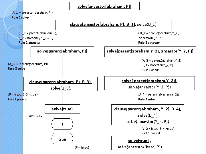
solve(ancestor(abraham, P)) {A_1 = ancestor(abraham, P)} Rule 3 solve clause(ancestor(abraham, P), B_1), solve(B_1) { B_1 = parent(abraham, P), X_2 = abraham, Y_2 = P } Rule 1 ancestor { B_1 = parent(abraham, Y_2), ancestor(Y_2, P) } Rule 2 ancestor solve(parent(abraham, P)) solve(parent(abraham, Y_2), ancestor(Y_2, P)) {A_3 = parent(abraham, Y_2) B_3 = ancestor(Y_2, P} Rule 2 solve {A_3 = parent(abraham, P)} Rule 3 solve clause(parent(abraham, P), B_3), solve(B_3). {P = issac, B_3 =true} Fact 1 parent solve( parent(abraham, Y_2)), solve(ancestor(Y_2, P)) {A_4 = parent(abraham, Y_2)} Rule 3 solve clause(parent(abraham, Y_2), B_4), solve(B_4) solve(ancestor(Y_2, P)) solve(true) Fact 1 solve ! {Y_2 = issac, B_4 =true} Fact 1 parent true {P = issac} solve(true) , solve(ancestor(issac, P))

Meta-Circular Interpreter Version 2 �In this version we control the goal selection order by using a stack of goals �Preprocessing – The given program is converted into a program with a single predicate rule containing only facts �Queries are checked against the new program

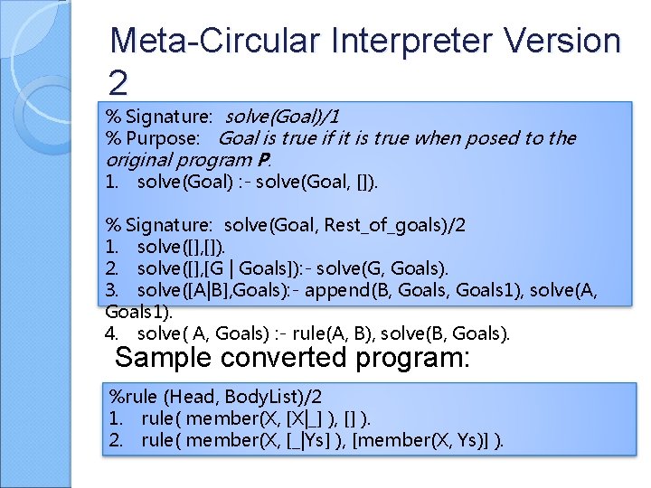
Meta-Circular Interpreter Version 2 % Signature: solve(Goal)/1 % Purpose: Goal is true if it is true when posed to the original program P. 1. solve(Goal) : - solve(Goal, []). % Signature: solve(Goal, Rest_of_goals)/2 1. solve([], []). 2. solve([], [G | Goals]): - solve(G, Goals). 3. solve([A|B], Goals): - append(B, Goals 1), solve(A, Goals 1). 4. solve( A, Goals) : - rule(A, B), solve(B, Goals). Sample converted program: %rule (Head, Body. List)/2 1. rule( member(X, [X|_] ), [] ). 2. rule( member(X, [_|Ys] ), [member(X, Ys)] ).

solve(member(X, [a, b, c])) {Goal_1 = member(X, [a, b, c])} Rule 1 solve(member(X, [a, b, c]), []) { A_2 = member(X, [a, b, c], Goals_1 = [] } Rule 4 solve rule(member(X, [a, b, c], B_2), solve(B_2, []) { X_3=X, Ys_3=[b, c], B_2 = [member(X, [b, c])]} Rule 2 rule { X=a, X_3 = a, Xs_3=[b, c], B_2 = [] } Rule 1 rule solve([], []) solve([member(X, [b, c])], []) Rule 1 solve { A_4= member(X, [b, c]), B_4=[], Goals_4=[] } Rule 3 rule true append([], Goals 1_4), solve(member(X, [b, c]), Goals 1_4). {X=a} { Goals 1_4=[]} Rule of append solve(member(X, [b, c]), []). { A_5=member(X, [b, c]), Goals_5=[]} Rule 4 solve rule(member(X, [b, c]), B_5), solve(B_5, []) { X=b, X_6 = b, B_5 = [] } Rule 1 rule solve([], []) Rule 1 solve true {X=b}