Logic for Computer Science Computing Math 1090 EECS

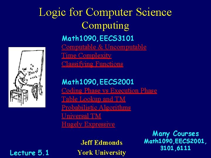
Logic for Computer Science Computing Math 1090, EECS 3101 Computable & Uncomputable Time Complexity Classifying Functions Lecture 5. 1 Math 1090, EECS 2001 Coding Phase vs Execution Phase Table Lookup and TM Probabilistic Algorithms Universal TM Hugely Expressive Many Courses Math 1090, EECS 2001, Jeff Edmonds 3101, 6111 York University

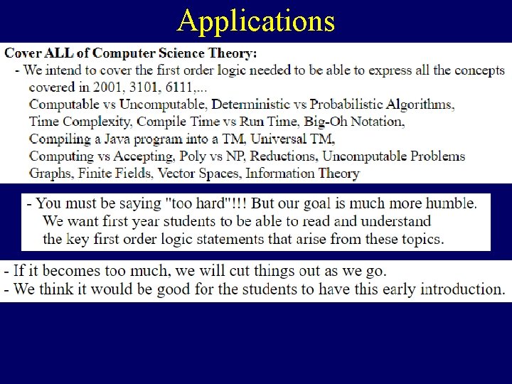
Applications

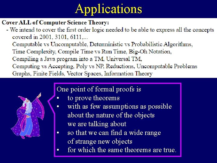
Applications One point of formal proofs is • to prove theorems • with as few assumptions as possible about the nature of the objects we are talking about • so that we can find a wide range of strange new objects • for which the same theorems are true.

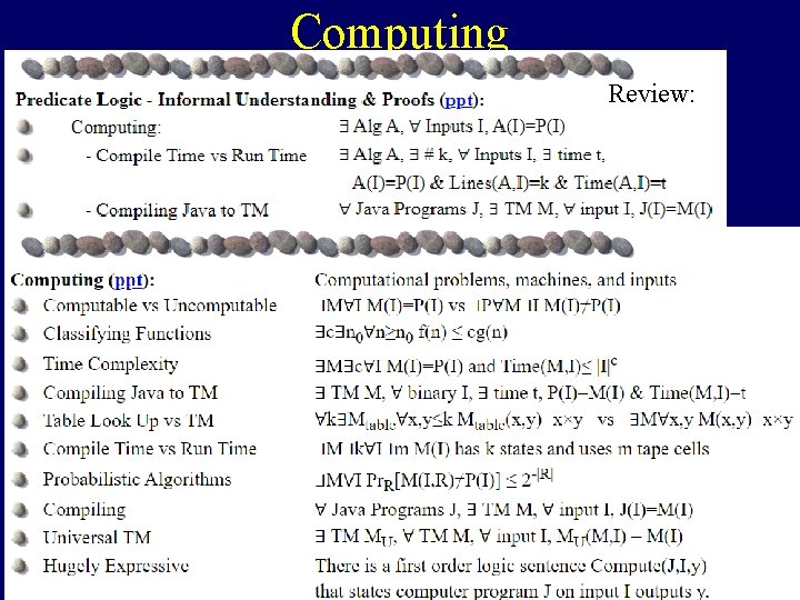
Computing Review:

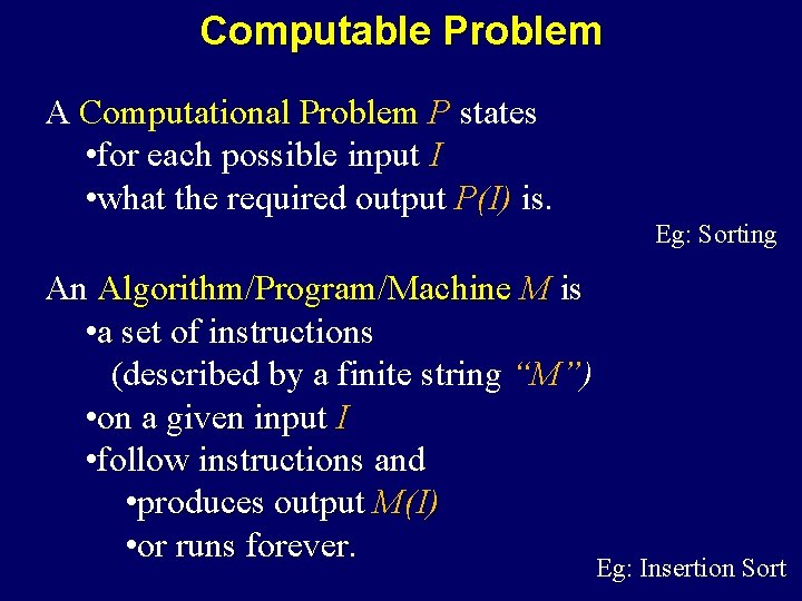
Computable Problem A Computational Problem P states • for each possible input I • what the required output P(I) is. Eg: Sorting An Algorithm/Program/Machine M is • a set of instructions (described by a finite string “M”) • on a given input I • follow instructions and • produces output M(I) • or runs forever. Eg: Insertion Sort

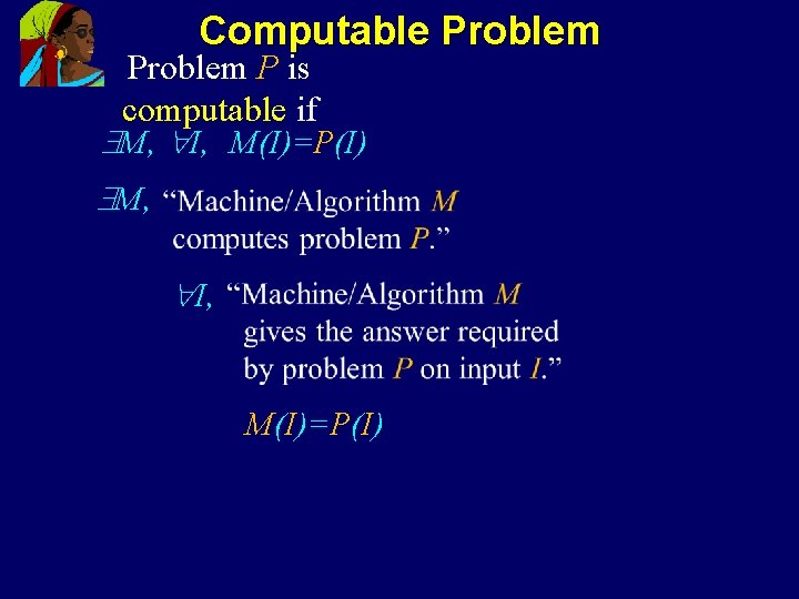
Computable Problem P is computable if M, I, M(I)=P(I) M, I, M(I)=P(I)

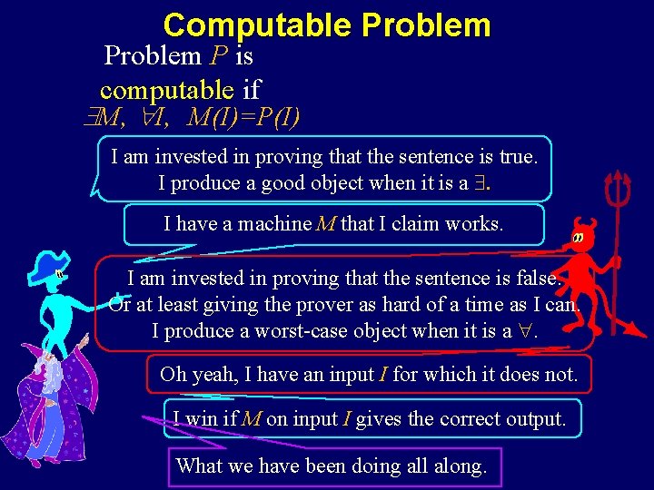
Computable Problem P is computable if M, I, M(I)=P(I) I am invested in proving that the sentence is true. I produce a good object when it is a . I have a machine M that I claim works. I am invested in proving that the sentence is false. Or at least giving the prover as hard of a time as I can. I produce a worst-case object when it is a . Oh yeah, I have an input I for which it does not. I win if M on input I gives the correct output. What we have been doing all along.

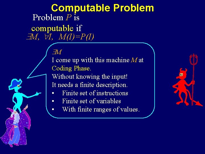
Computable Problem P is computable if M, I, M(I)=P(I) M I come up with this machine M at Coding Phase. Without knowing the input! It needs a finite description. • Finite set of instructions • Finite set of variables • With finite ranges of values.

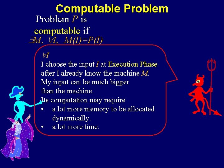
Computable Problem P is computable if M, I, M(I)=P(I) I I choose the input I at Execution Phase after I already know the machine M. My input can be much bigger than the machine. Its computation may require • a lot more memory to be allocated dynamically. • a lot more time.

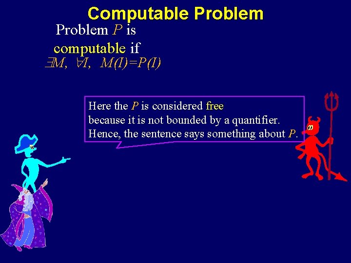
Computable Problem P is computable if M, I, M(I)=P(I) Here the P is considered free because it is not bounded by a quantifier. Hence, the sentence says something about P.

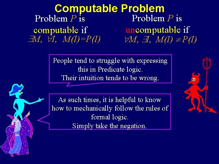
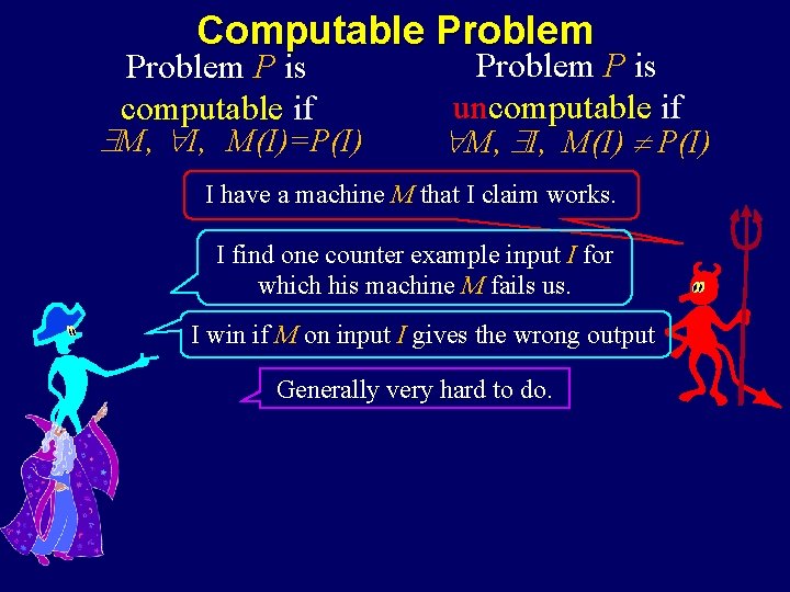
Computable Problem P is computable if M, I, M(I)=P(I) Problem P is uncomputable if M, I, M(I) P(I) People tend to struggle with expressing this in Predicate logic. Their intuition tends to be wrong. As such times, it is helpful to know how to mechanically follow the rules of formal logic. Simply take the negation.

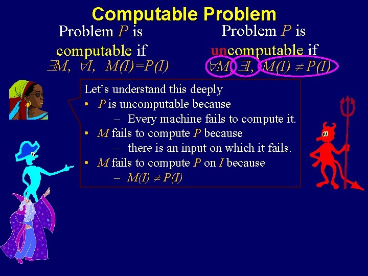
Computable Problem P is computable if M, I, M(I)=P(I) Problem P is uncomputable if M, I, M(I) P(I) Let’s understand this deeply • P is uncomputable because – Every machine fails to compute it. • M fails to compute P because – there is an input on which it fails. • M fails to compute P on I because – M(I) P(I)

Computable Problem P is computable if M, I, M(I)=P(I) Problem P is uncomputable if M, I, M(I) P(I) I have a machine M that I claim works. I find one counter example input I for which his machine M fails us. I win if M on input I gives the wrong output Generally very hard to do.

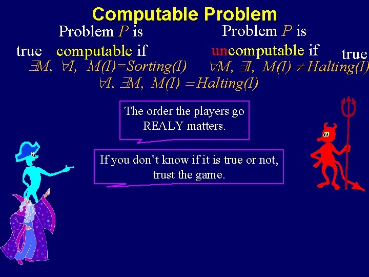
Computable Problem P is uncomputable if true computable if M, I, M(I)=Sorting(I) M, I, M(I) Halting(I) I, M, M(I) = Halting(I) The order the players go REALY matters. If you don’t know if it is true or not, trust the game.

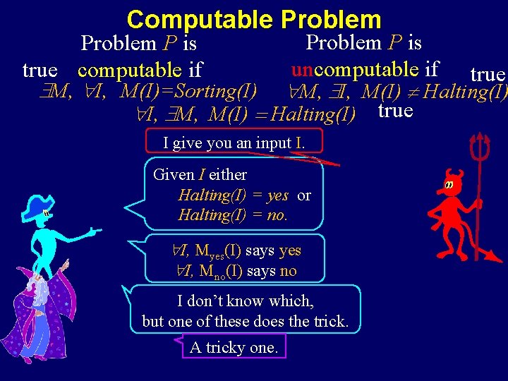
Computable Problem P is uncomputable if true computable if M, I, M(I)=Sorting(I) M, I, M(I) Halting(I) I, M, M(I) = Halting(I) true I give you an input I. Given I either Halting(I) = yes or Halting(I) = no. I, Myes(I) says yes I, Mno(I) says no I don’t know which, but one of these does the trick. A tricky one.

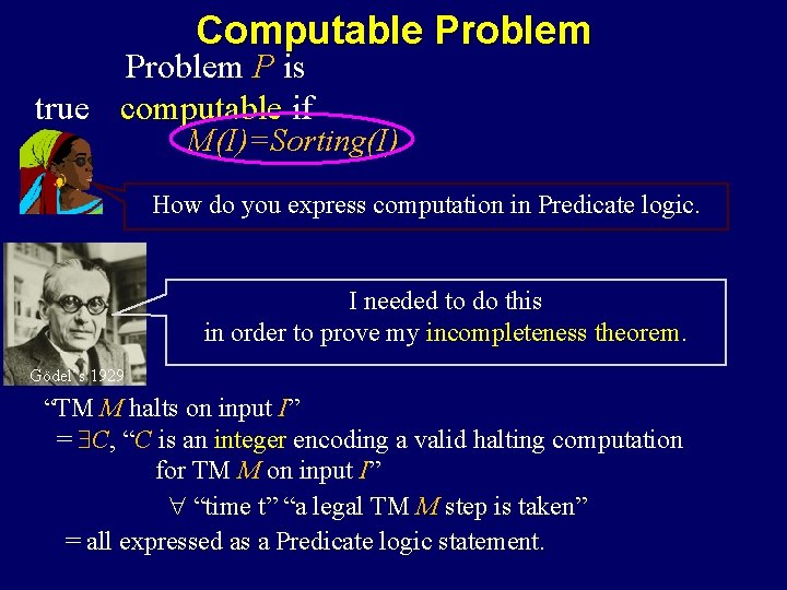
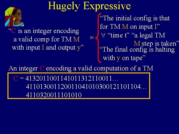
Computable Problem P is true computable if M(I)=Sorting(I) How do you express computation in Predicate logic. I needed to do this in order to prove my incompleteness theorem. Gödel’s 1929 “TM M halts on input I” “ = C, “C is an integer encoding a valid halting computation for TM M on input I” “time t” “a legal TM M step is taken” = all expressed as a Predicate logic statement.

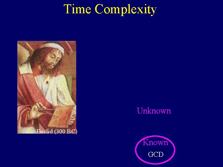
Time Complexity Unknown Euclid (300 BC) Known GCD

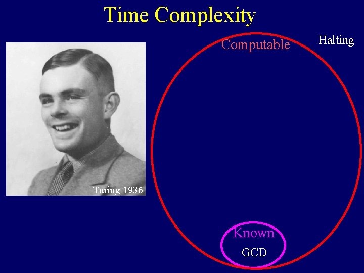
Time Complexity Computable Turing 1936 Known GCD Halting

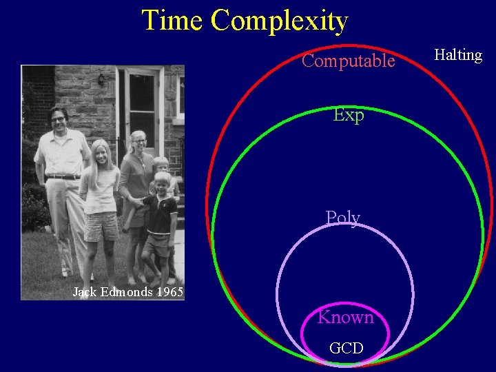
Time Complexity Computable Exp Poly Jack Edmonds 1965 Known GCD Halting

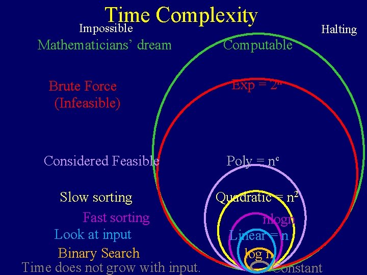
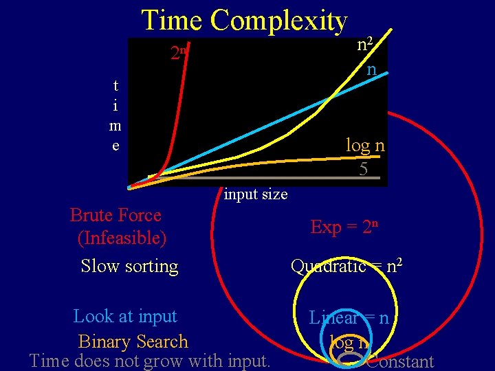
Time Complexity Impossible Mathematicians’ dream Brute Force (Infeasible) Considered Feasible Halting Computable Exp = 2 n Poly = nc Quadratic = n 2 Slow sorting Fast sorting nlogn Look at input Linear = n Binary Search log n Time does not grow with input. Constant

Time Complexity 2 n t i m e n 2 n log n 5 input size Brute Force (Infeasible) Slow sorting Look at input Binary Search Time does not grow with input. Exp = 2 n Quadratic = n 2 Linear = n log n Constant

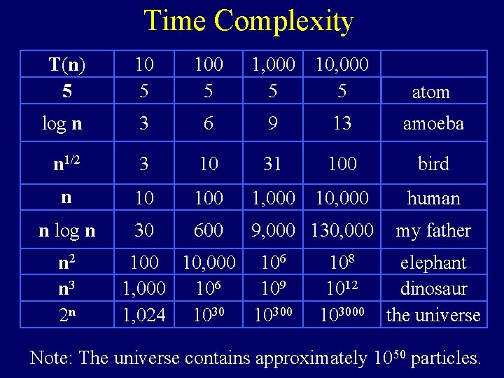
Time Complexity T(n) 5 100 5 1, 000 5 10, 000 5 atom log n 3 6 9 13 amoeba n 1/2 3 10 31 100 bird n 10 100 1, 000 10, 000 human n log n 30 600 9, 000 130, 000 n 2 n 3 2 n 100 10, 000 106 109 1, 024 10300 108 1012 103000 my father elephant dinosaur the universe Note: The universe contains approximately 1050 particles.

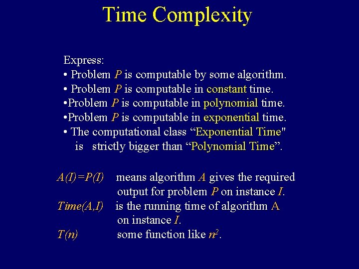
Time Complexity Express: • Problem P is computable by some algorithm. • Problem P is computable in constant time. • Problem P is computable in polynomial time. • Problem P is computable in exponential time. • The computational class “Exponential Time" is strictly bigger than “Polynomial Time”. A(I)=P(I) means algorithm A gives the required output for problem P on instance I. Time(A, I) is the running time of algorithm A on instance I. T(n) some function like n 2.

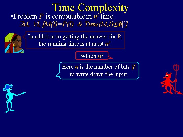
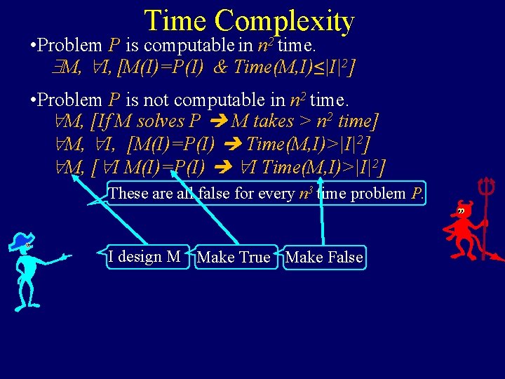
Time Complexity • Problem P is computable in n 2 time. M, I, [M(I)=P(I) & Time(M, I)≤|I| n 2] In addition to getting the answer for P, the running time is at most n 2. Which n? Here n is the number of bits |I| to write down the input.

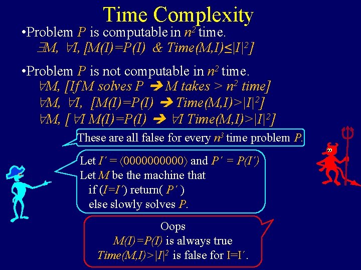
Time Complexity • Problem P is computable in n 2 time. M, I, [M(I)=P(I) & Time(M, I)≤|I|2] • Problem P is not computable in n 2 time. M, [If M solves P M takes > n 2 time] M, I, [M(I)=P(I) Time(M, I)>|I|2] M, [ I M(I)=P(I) I Time(M, I)>|I|2] These are all false for every n 3 time problem P. I design M Make True Make False

Time Complexity • Problem P is computable in n 2 time. M, I, [M(I)=P(I) & Time(M, I)≤|I|2] • Problem P is not computable in n 2 time. M, [If M solves P M takes > n 2 time] M, I, [M(I)=P(I) Time(M, I)>|I|2] M, [ I M(I)=P(I) I Time(M, I)>|I|2] These are all false for every n 3 time problem P. Let I´ = 00000 and P´ = P(I´) Let M be the machine that if (I=I´) return( P´ ) else slowly solves P. Oops M(I)=P(I) is always true Time(M, I)>|I|2 is false for I=I´.

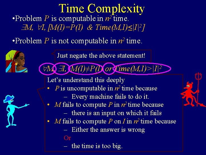
Time Complexity • Problem P is computable in n 2 time. M, I, [M(I)=P(I) & Time(M, I)≤|I|2] • Problem P is not computable in n 2 time. Just negate the above statement! M, I, M(I)≠P(I) or Time(M, I)>|I|2 Let’s understand this deeply • P is uncomputable in n 2 time because – Every machine fails to do it. • M fails to compute P in n 2 time because – there is an input on which it fails • M fails to compute P on I in n 2 time because – Either the answer is wrong Or – the time is too big.

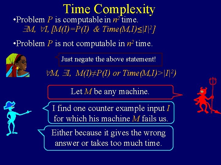
Time Complexity • Problem P is computable in n 2 time. M, I, [M(I)=P(I) & Time(M, I)≤|I|2] • Problem P is not computable in n 2 time. Just negate the above statement! M, I, M(I)≠P(I) or Time(M, I)>|I|2) Let M be any machine. I find one counter example input I for which his machine M fails us. Either because it gives the wrong answer or takes too much time.

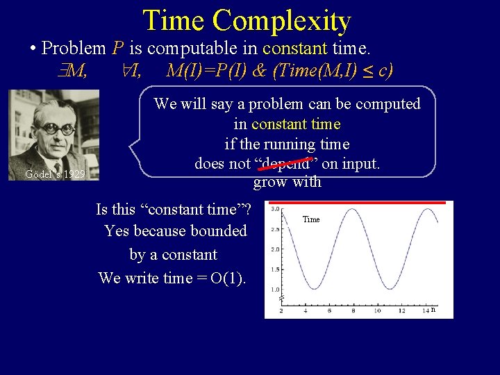
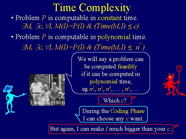
Time Complexity • Problem P is computable in constant time. M, I, M(I)=P(I) & (Time(M, I) ≤ c) Gödel’s 1929 We will say a problem can be computed in constant time if the running time does not “depend” on input. grow with Is this “constant time”? Yes because bounded by a constant We write time = O(1). Time n

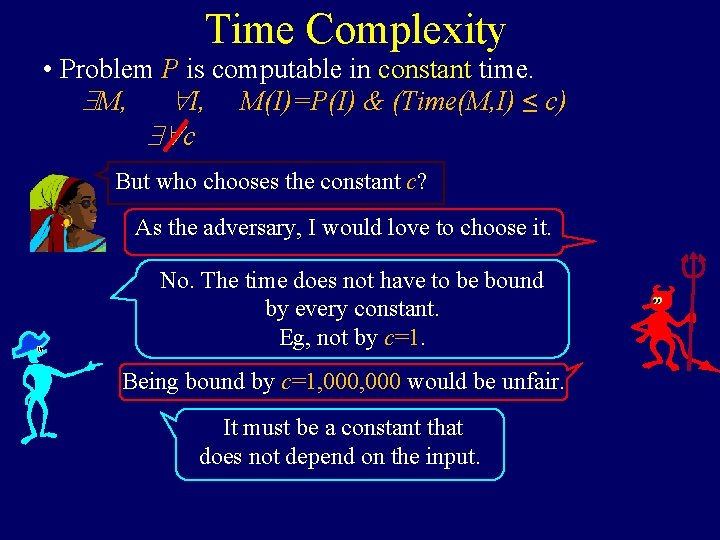
Time Complexity • Problem P is computable in constant time. M, I, M(I)=P(I) & (Time(M, I) ≤ c) c But who chooses the constant c? As the adversary, I would love to choose it. No. The time does not have to be bound by every constant. Eg, not by c=1. Being bound by c=1, 000 would be unfair. It must be a constant that does not depend on the input.

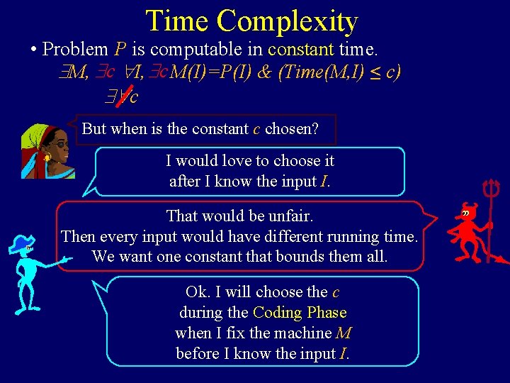
Time Complexity • Problem P is computable in constant time. M, c I, c M(I)=P(I) & (Time(M, I) ≤ c) c But when is the constant c chosen? I would love to choose it after I know the input I. That would be unfair. Then every input would have different running time. We want one constant that bounds them all. Ok. I will choose the c during the Coding Phase when I fix the machine M before I know the input I.

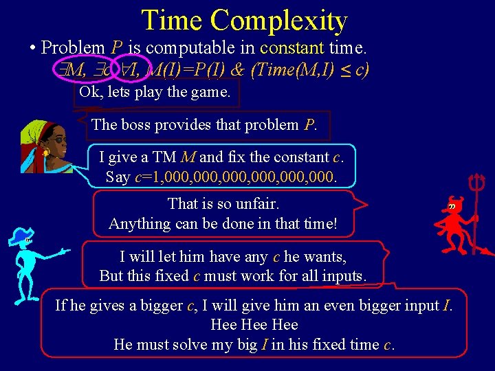
Time Complexity • Problem P is computable in constant time. M, c, I, M(I)=P(I) & (Time(M, I) ≤ c) Ok, lets play the game. The boss provides that problem P. I give a TM M and fix the constant c. Say c=1, 000, 000. That is so unfair. Anything can be done in that time! I will let him have any c he wants, But this fixed c must work for all inputs. If he gives a bigger c, I will give him an even bigger input I. Hee Hee He must solve my big I in his fixed time c.

Time Complexity • Problem P is computable in constant time. M, c, I, M(I)=P(I) & (Time(M, I) ≤ c) • Problem P is computable in polynomial time. c M, c, I, M(I)=P(I) & (Time(M, I) ≤ n ) We will say a problem can be computed feasibly if it can be computed in polynomial time, eg n 2, n 3, n 4, … , nc, … Edmonds (1963) Which c? During the Coding Phase I can choose any c want. But again, I can make I much bigger than your c.

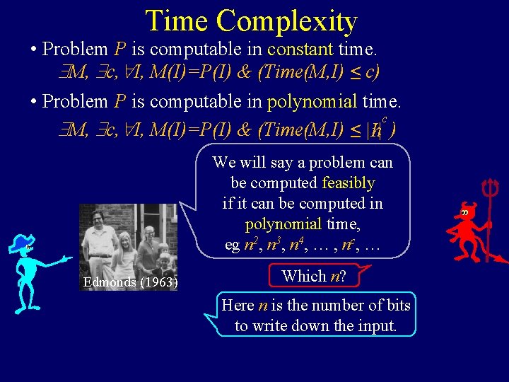
Time Complexity • Problem P is computable in constant time. M, c, I, M(I)=P(I) & (Time(M, I) ≤ c) • Problem P is computable in polynomial time. c M, c, I, M(I)=P(I) & (Time(M, I) ≤ |I|n ) We will say a problem can be computed feasibly if it can be computed in polynomial time, eg n 2, n 3, n 4, … , nc, … Edmonds (1963) Which n? Here n is the number of bits to write down the input.

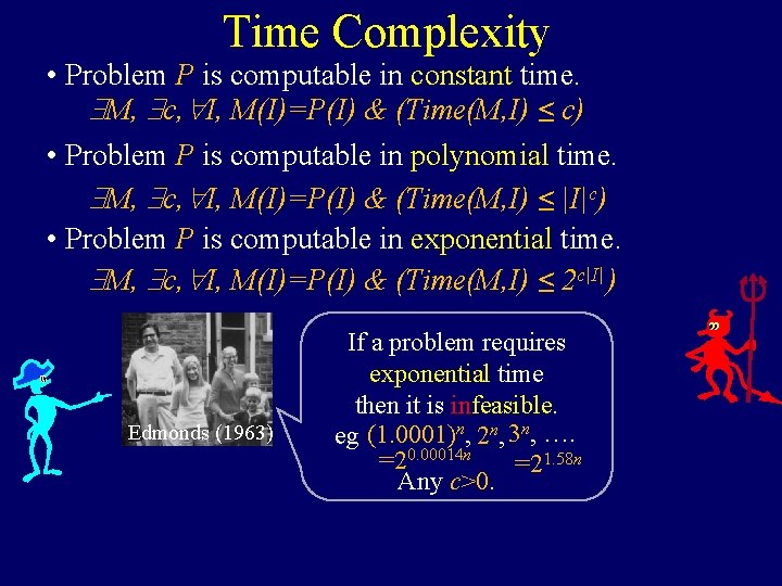
Time Complexity • Problem P is computable in constant time. M, c, I, M(I)=P(I) & (Time(M, I) ≤ c) • Problem P is computable in polynomial time. M, c, I, M(I)=P(I) & (Time(M, I) ≤ |I|c) • Problem P is computable in exponential time. M, c, I, M(I)=P(I) & (Time(M, I) ≤ 2 c|I| ) Edmonds (1963) If a problem requires exponential time then it is infeasible. (1. 0001)n, n, 3 n, …. eg 2 =20. 00014 n =21. 58 n Any c>0.

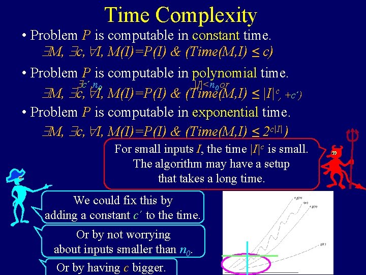
Time Complexity • Problem P is computable in constant time. M, c, I, M(I)=P(I) & (Time(M, I) ≤ c) • Problem P is computable in polynomial time. c´, n 0, |I|<n 0 or M, c, I, M(I)=P(I) & (Time(M, I) ≤ |I|c)+c´) • Problem P is computable in exponential time. M, c, I, M(I)=P(I) & (Time(M, I) ≤ 2 c|I| ) For small inputs I, the time |I|c is small. The algorithm may have a setup that takes a long time. We could fix this by adding a constant c´ to the time. Or by not worrying about inputs smaller than n 0. Or by having c bigger.

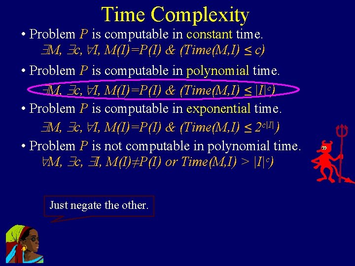
Time Complexity • Problem P is computable in constant time. M, c, I, M(I)=P(I) & (Time(M, I) ≤ c) • Problem P is computable in polynomial time. M, c, I, M(I)=P(I) & (Time(M, I) ≤ |I|c) • Problem P is computable in exponential time. M, c, I, M(I)=P(I) & (Time(M, I) ≤ 2 c|I| ) • Problem P is not computable in polynomial time. M, c, I, M(I)≠P(I) or Time(M, I) > |I|c) Just negate the other.

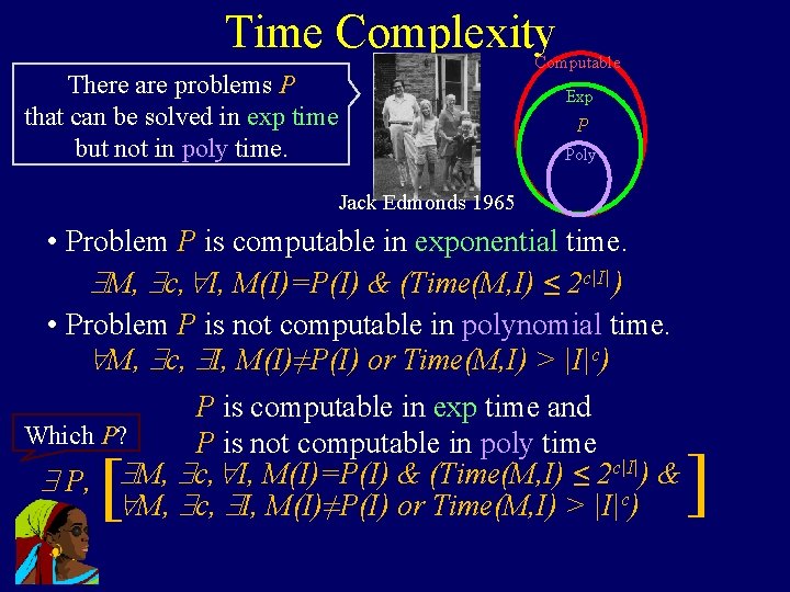
Time Complexity Computable There are problems P that can be solved in exp time but not in poly time. Exp P Poly Jack Edmonds 1965 • Problem P is computable in exponential time. M, c, I, M(I)=P(I) & (Time(M, I) ≤ 2 c|I| ) • Problem P is not computable in polynomial time. M, c, I, M(I)≠P(I) or Time(M, I) > |I|c) P is computable in exp time and Which P? P is not computable in poly time c|I|) & M, c, I, M(I)=P(I) & (Time(M, I) ≤ 2 P, M, c, I, M(I)≠P(I) or Time(M, I) > |I|c) [ ]

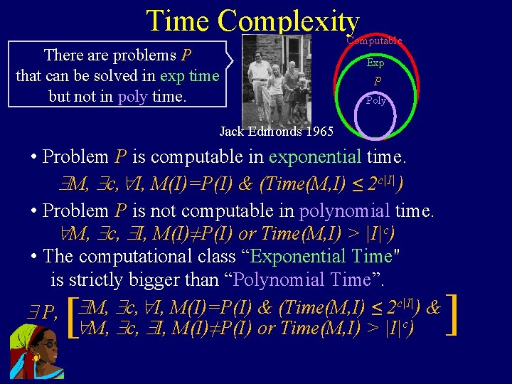
Time Complexity Computable There are problems P that can be solved in exp time but not in poly time. Exp P Poly Jack Edmonds 1965 • Problem P is computable in exponential time. M, c, I, M(I)=P(I) & (Time(M, I) ≤ 2 c|I| ) • Problem P is not computable in polynomial time. M, c, I, M(I)≠P(I) or Time(M, I) > |I|c) • The computational class “Exponential Time" is strictly bigger than “Polynomial Time”. c|I|) & M, c, I, M(I)=P(I) & (Time(M, I) ≤ 2 P, M, c, I, M(I)≠P(I) or Time(M, I) > |I|c) [ ]

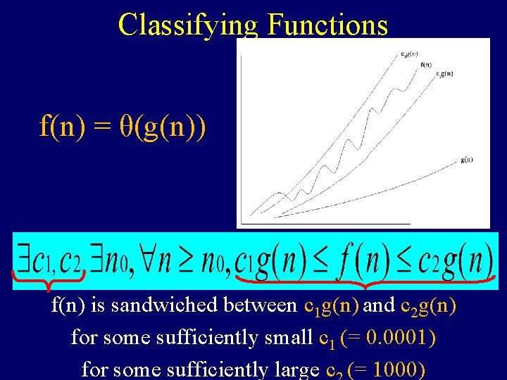
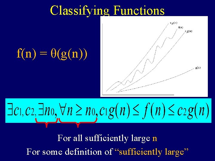
Classifying Functions f(n) = θ(g(n)) f(n) is sandwiched between c 1 g(n) and c 2 g(n) for some sufficiently small c 1 (= 0. 0001) for some sufficiently large c (= 1000)

Classifying Functions f(n) = θ(g(n)) For all sufficiently large n For some definition of “sufficiently large”

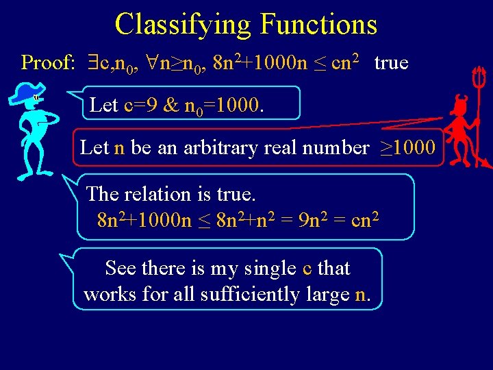
Classifying Functions Proof: c, n 0, n≥n 0, 8 n 2+1000 n ≤ cn 2 true Let c=9 & n 0=1000. Let n be an arbitrary real number ≥ 1000 The relation is true. 8 n 2+1000 n ≤ 8 n 2+n 2 = 9 n 2 = cn 2 See there is my single c that works for all sufficiently large n.

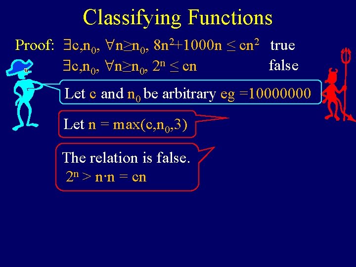
Classifying Functions Proof: c, n 0, n≥n 0, 8 n 2+1000 n ≤ cn 2 true false c, n 0, n≥n 0, 2 n ≤ cn Let c and n 0 be arbitrary eg =10000000 Let n = max(c, n 0, 3) The relation is false. 2 n > n∙n = cn

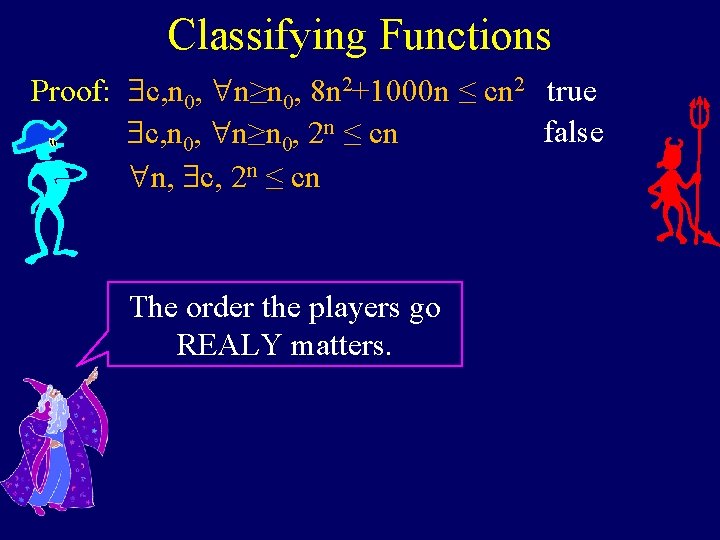
Classifying Functions Proof: c, n 0, n≥n 0, 8 n 2+1000 n ≤ cn 2 true false c, n 0, n≥n 0, 2 n ≤ cn n, c, 2 n ≤ cn The order the players go REALY matters.

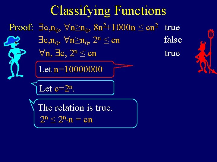
Classifying Functions Proof: c, n 0, n≥n 0, 8 n 2+1000 n ≤ cn 2 true false c, n 0, n≥n 0, 2 n ≤ cn n, c, 2 n ≤ cn true Let n=10000000 Let c=2 n. The relation is true. 2 n ≤ 2 n n = cn

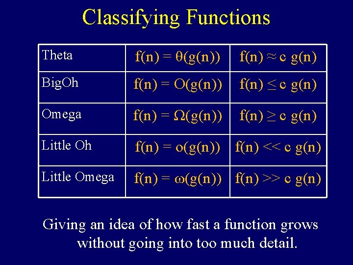
Classifying Functions Theta f(n) = θ(g(n)) f(n) ≈ c g(n) Big. Oh f(n) = O(g(n)) f(n) ≤ c g(n) Omega f(n) = Ω(g(n)) f(n) ≥ c g(n) Little Oh f(n) = o(g(n)) f(n) << c g(n) Little Omega f(n) = ω(g(n)) f(n) >> c g(n) Giving an idea of how fast a function grows without going into too much detail.

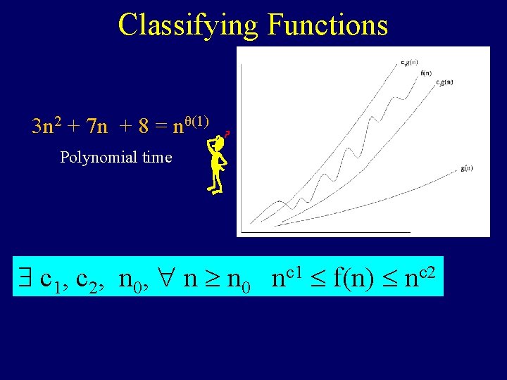
Classifying Functions 3 n 2 + 7 n + 8 = nθ(1) Polynomial time c 1, c 2, n 0, n ³ n 0 nc 1 f(n) nc 2

Classifying Functions 3 n n = 2[ log(3) n + log n ] = 2θ(n) Exponential time c 1, c 2, n 0, n ³ n 0 2 c 1 n f(n) 2 c 2 n

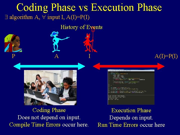
Coding Phase vs Execution Phase algorithm A, input I, A(I)=P(I) History of Events P A I Coding Phase Does not depend on input. Compile Time Errors occur here. A(I)=P(I) Execution Phase Depends on input. Run Time Errors occur here

Coding Phase vs Execution Phase algorithm A, input I, A(I)=P(I) For more, see Math 1090 slides Informal Understanding & Informal Proofs

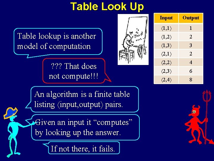
Table Look Up Table lookup is another model of computation ? ? ? That does not compute!!! An algorithm is a finite table listing input, output pairs. Given an input it “computes” by looking up the answer. If not there, it fails. Input Output 1, 1 1 1, 2 2 1, 3 3 2, 1 2 2, 2 4 2, 3 6 2, 4 8

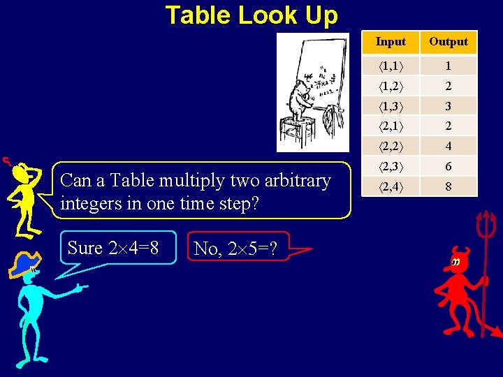
Table Look Up Can a Table multiply two arbitrary integers in one time step? Sure 2 4=8 No, 2 5=? Input Output 1, 1 1 1, 2 2 1, 3 3 2, 1 2 2, 2 4 2, 3 6 2, 4 8

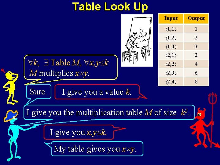
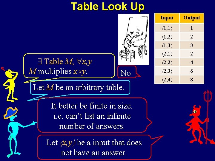
Table Look Up k, Table M, x, y k M multiplies x y. Sure. Input Output 1, 1 1 1, 2 2 1, 3 3 2, 1 2 2, 2 4 2, 3 6 2, 4 8 I give you a value k. I give you the multiplication table M of size k 2. I give you x, y k. My table gives you x y.

Table Look Up Table M, x, y M multiplies x y. No Let M be an arbitrary table. It better be finite in size. i. e. can’t list an infinite number of answers. Let x, y be a input that does not have an answer. Input Output 1, 1 1 1, 2 2 1, 3 3 2, 1 2 2, 2 4 2, 3 6 2, 4 8

Probabilistic Algorithms

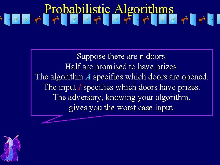
Probabilistic Algorithms Suppose there are n doors. Half are promised to have prizes. The algorithm A specifies which doors are opened. The input I specifies which doors have prizes. The adversary, knowing your algorithm, gives you the worst case input.

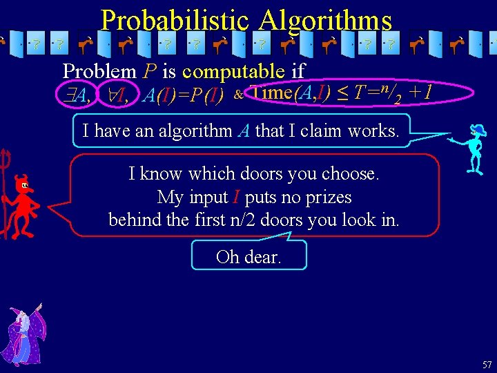
Probabilistic Algorithms Problem P is computable if A, I, A(I)=P(I) & Time(A, I) ≤ T =n/2 +1 I have an algorithm A that I claim works. I know which doors you choose. My input I puts no prizes behind the first n/2 doors you look in. Oh dear. 57

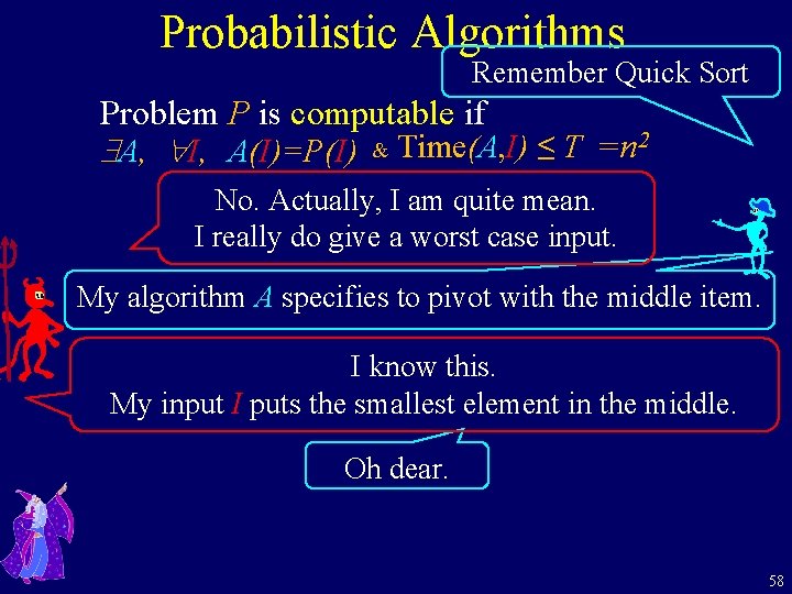
Probabilistic Algorithms Remember Quick Sort Problem P is computable if A, I, A(I)=P(I) & Time(A, I) ≤ T =n 2 No. Actually, I am quite mean. I really do give a worst case input. My algorithm A specifies to pivot with the middle item. I know this. My input I puts the smallest element in the middle. Oh dear. 58

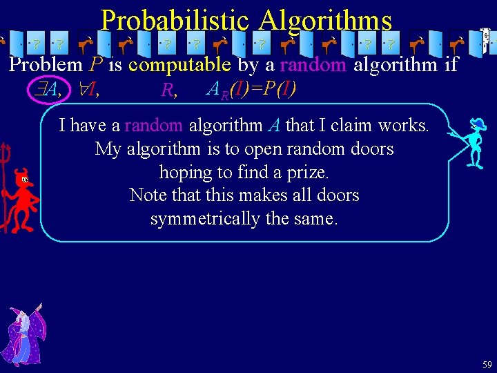
Probabilistic Algorithms Problem P is computable by a random algorithm if A, I, R, AR(I)=P(I) I have a random algorithm A that I claim works. My algorithm is to open random doors hoping to find a prize. Note that this makes all doors symmetrically the same. 59

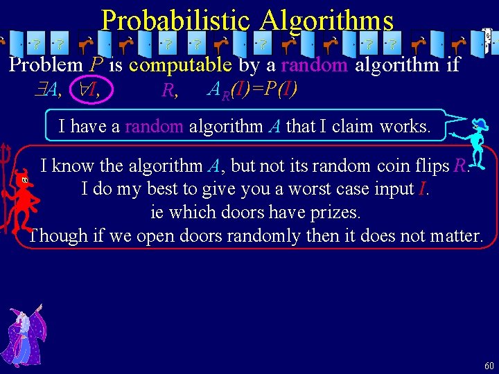
Probabilistic Algorithms Problem P is computable by a random algorithm if A, I, R, AR(I)=P(I) I have a random algorithm A that I claim works. I know the algorithm A, but not its random coin flips R. I do my best to give you a worst case input I. ie which doors have prizes. Though if we open doors randomly then it does not matter. 60

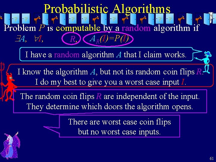
Probabilistic Algorithms Problem P is computable by a random algorithm if A, I, R, AR(I)=P(I) I have a random algorithm A that I claim works. I know the algorithm A, but not its random coin flips R. I do my best to give you a worst case input I. The random coin flips R are independent of the input. They determine which doors the algorithm opens. There are worst case coin flips but no worst case inputs. 61

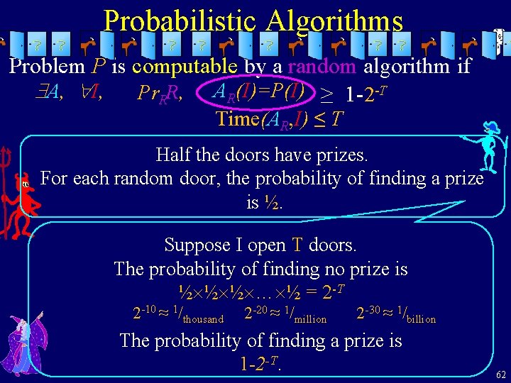
Probabilistic Algorithms Problem P is computable by a random algorithm if A, I, Pr. RR, AR(I)=P(I) ≥ 1 -2 -T Time(AR, I) ≤ T Half the doors have prizes. For each random door, the probability of finding a prize is ½. Suppose I open T doors. The probability of finding no prize is ½ ½ ½ … ½ = 2 -T 2 -10 ≈ 1/thousand 2 -20 ≈ 1/million 2 -30 ≈ 1/billion The probability of finding a prize is 1 -2 -T. 62

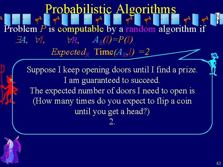
Probabilistic Algorithms Problem P is computable by a random algorithm if A, I, R, AR(I)=P(I) Expected. R Time(AR, I) =2 Suppose I keep opening doors until I find a prize. I am guaranteed to succeed. The expected number of doors I need to open is (How many times do you expect to flip a coin until you get a head? ) 2. 63

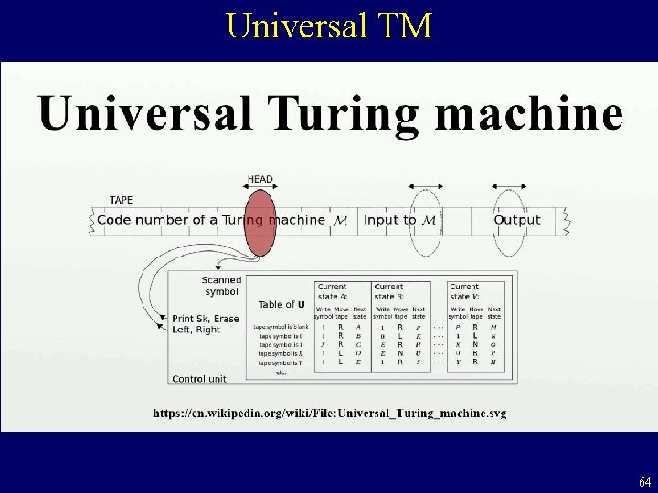
Universal TM 64

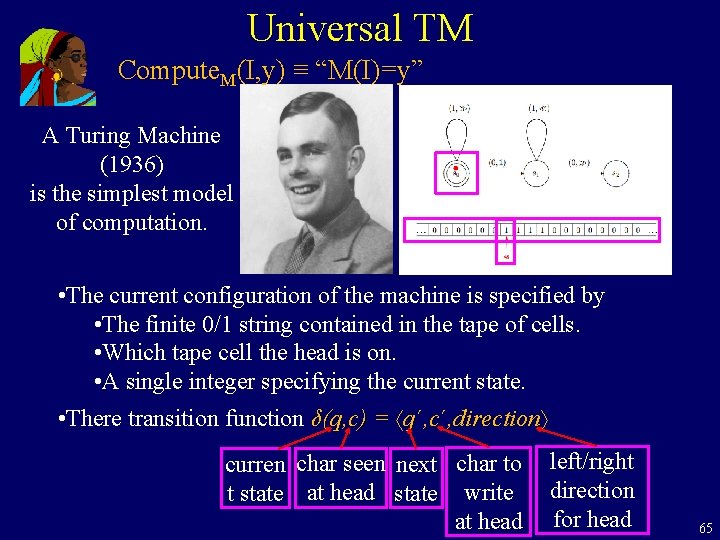
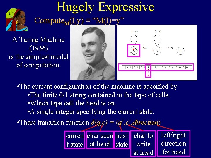
Universal TM Compute. M(I, y) ≡ “M(I)=y” A Turing Machine (1936) is the simplest model of computation. • The current configuration of the machine is specified by • The finite 0/1 string contained in the tape of cells. • Which tape cell the head is on. • A single integer specifying the current state. • There transition function δ(q, c) = q´, c´ , c , direction curren char seen next char to left/right direction t state at head state write at head for head 65

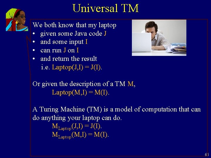
Universal TM We both know that my laptop • given some Java code J • and some input I • can run J on I • and return the result i. e. Laptop(J, I) = J(I). Or given the description of a TM M, Laptop(M, I) = M(I). A Turing Machine (TM) is a model of computation that can do anything your laptop can do. MLaptop(J, I) = J(I). MLaptop(M, I) = M(I). 66

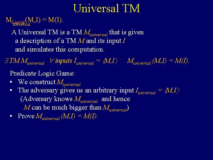
Universal TM MLaptop(M, I) = M(I). universal A Universal TM is a TM Muniversal that is given a description of a TM M and its input I and simulates this computation. TM Muniversal inputs Iuniversal = M, I Muniversal (M, I) = M(I). Predicate Logic Game: • We construct Muniversal • The adversary gives us an arbitrary input Iuniversal = M, I (Adversary knows Muniversal and hence M can be much bigger than Muniversal) • Prove Muniversal (M, I) = M(I).

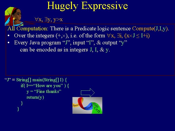
Hugely Expressive x, y, y>x Predicate logic can only say these stupid things. Why should I care? Actually, it is hugely expressive. • Math: For any mathematical statement you want to understand prove, it is best to first write it as a Predicate logic sentence. • Proof: Sometimes the mechanics of the proof just falls out. • The next example is really quite amazing!

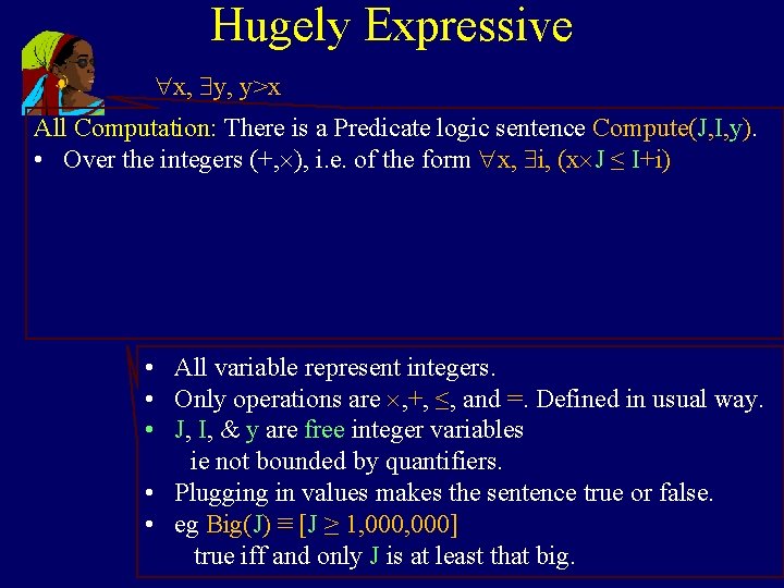
Hugely Expressive x, y, y>x All Computation: There is a Predicate logic sentence Compute(J, I, y). • Over the integers (+, ), i. e. of the form x, i, (x J ≤ I+i) • All variable represent integers. • Only operations are , +, ≤, and =. Defined in usual way. • J, I, & y are free integer variables ie not bounded by quantifiers. • Plugging in values makes the sentence true or false. • eg Big(J) ≡ [J ≥ 1, 000] true iff and only J is at least that big.

Hugely Expressive x, y, y>x All Computation: There is a Predicate logic sentence Compute(J, I, y). • Over the integers (+, ), i. e. of the form x, i, (x J ≤ I+i) • Every Java program “J”, input “I”, & output “y” can be encoded as in integers J, I, & y. “J” ≡ String[] main(String[] I) { if( I==“How are you” ) { y = “Fine thanks” return(y) } }

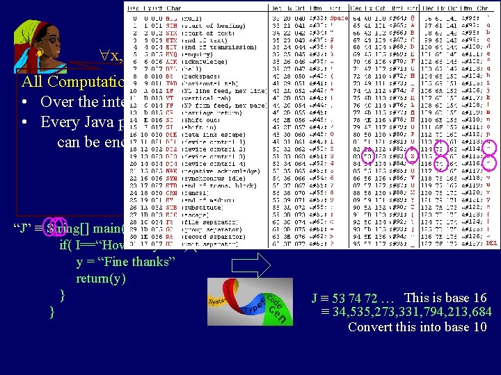
Hugely Expressive x, y, y>x All Computation: There is a Predicate logic sentence Compute(J, I, y). • Over the integers (+, ), i. e. of the form x, i, (x J ≤ I+i) • Every Java program “J”, input “I”, & output “y” can be encoded as in integers J, I, & y. “J” ≡ String[] main(String[] I) { if( I==“How are you” ) { y = “Fine thanks” return(y) } } J ≡ 53 74 72 … This is base 16 ≡ 34, 535, 273, 331, 794, 213, 684 Convert this into base 10

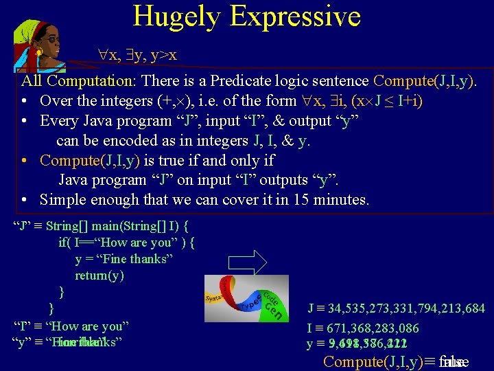
Hugely Expressive x, y, y>x All Computation: There is a Predicate logic sentence Compute(J, I, y). • Over the integers (+, ), i. e. of the form x, i, (x J ≤ I+i) • Every Java program “J”, input “I”, & output “y” can be encoded as in integers J, I, & y. • Compute(J, I, y) is true if and only if Java program “J” on input “I” outputs “y”. • Simple enough that we can cover it in 15 minutes. “J” ≡ String[] main(String[] I) { if( I==“How are you” ) { y = “Fine thanks” return(y) } } “I” ≡ “How are you” “y” ≡ “Horrible” “y” ≡ “Fine thanks” J ≡ 34, 535, 273, 331, 794, 213, 684 I ≡ 671, 368, 283, 086 y ≡ 9, 418, 386, 212 y ≡ 3, 691, 576, 421 ≡ true Compute(J, I, y) ≡ false

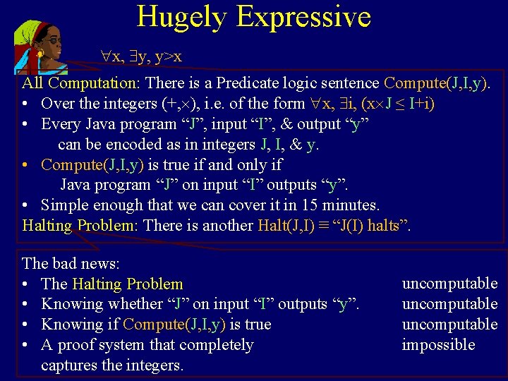
Hugely Expressive x, y, y>x All Computation: There is a Predicate logic sentence Compute(J, I, y). • Over the integers (+, ), i. e. of the form x, i, (x J ≤ I+i) • Every Java program “J”, input “I”, & output “y” can be encoded as in integers J, I, & y. • Compute(J, I, y) is true if and only if Java program “J” on input “I” outputs “y”. • Simple enough that we can cover it in 15 minutes. Halting Problem: There is another Halt(J, I) ≡ “J(I) halts”. The bad news: • The Halting Problem • Knowing whether “J” on input “I” outputs “y”. • Knowing if Compute(J, I, y) is true • A proof system that completely captures the integers. uncomputable impossible

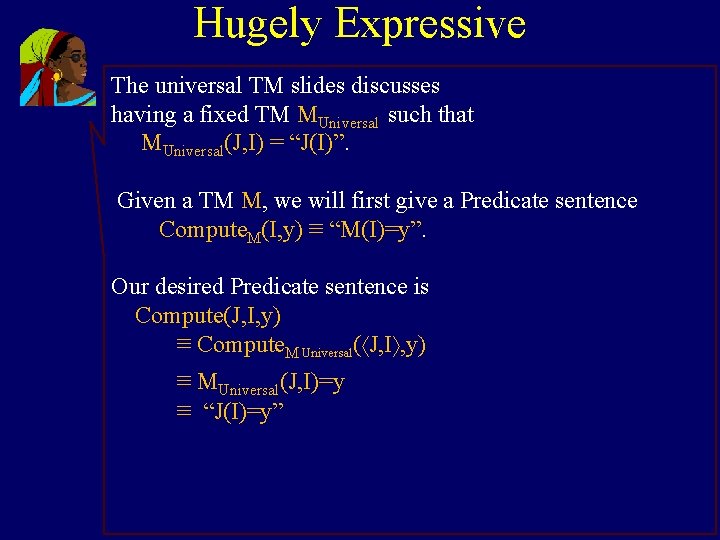
Hugely Expressive The universal TM slides discusses having a fixed TM MUniversal such that MUniversal(J, I) = “J(I)”. Given a TM M, we will first give a Predicate sentence Compute. M(I, y) ≡ “M(I)=y”. Our desired Predicate sentence is Compute(J, I, y) ≡ Compute. M ( J, I , y) Universal ≡ MUniversal(J, I)=y ≡ “J(I)=y”

Hugely Expressive Compute. M(I, y) ≡ “M(I)=y” A Turing Machine (1936) is the simplest model of computation. • The current configuration of the machine is specified by • The finite 0/1 string contained in the tape of cells. • Which tape cell the head is on. • A single integer specifying the current state. • There transition function δ(q, c) = q´, c´ , c , direction curren char seen next char to left/right direction t state at head state write at head for head

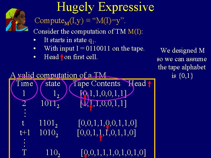
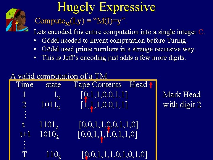
Hugely Expressive Compute. M(I, y) ≡ “M(I)=y”. Consider the computation of TM M(I): • It starts in state q 1. • With input I = 0110011 on the tape. • Head on first cell. … A valid computation of a TM Time state Tape Contents Head 1 12 [0, 1, 1, 0, 0, 1, 1] 2 10112 [1, 1, 1, 0, 0, 1, 1] … t 11012 [0, 0, 1, 1, 0] t+1 10102 [0, 0, 1, 1, 1, 0] T 1102 [0, 0, 1, 1, 1, 0, 1, 0] We designed M so we can assume the tape alphabet is {0, 1}

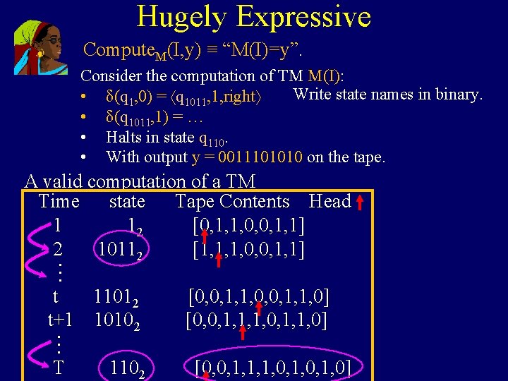
Hugely Expressive Compute. M(I, y) ≡ “M(I)=y”. Consider the computation of TM M(I): Write state names in binary. • δ(q 1, 0) = q 1011, 1, right • δ(q 1011, 1) = … • Halts in state q 110. • With output y = 0011101010 on the tape. … A valid computation of a TM Time state Tape Contents Head 1 12 [0, 1, 1, 0, 0, 1, 1] 2 10112 [1, 1, 1, 0, 0, 1, 1] … t 11012 [0, 0, 1, 1, 0] t+1 10102 [0, 0, 1, 1, 1, 0] T 1102 [0, 0, 1, 1, 1, 0, 1, 0]

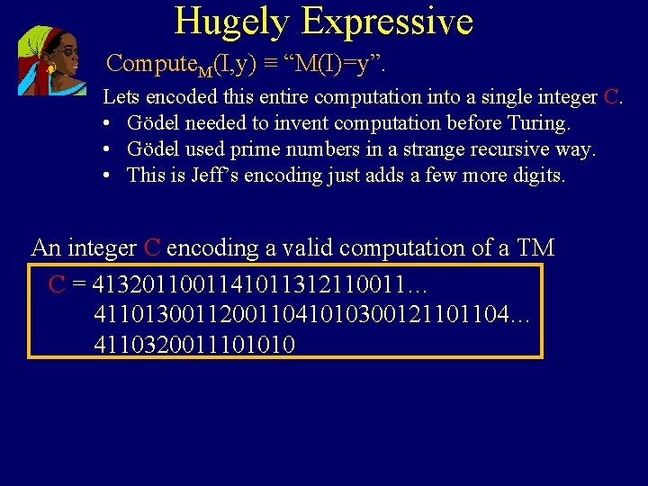
Hugely Expressive Compute. M(I, y) ≡ “M(I)=y”. Lets encoded this entire computation into a single integer C. • Gödel needed to invent computation before Turing. • Gödel used prime numbers in a strange recursive way. • This is Jeff’s encoding just adds a few more digits. … A valid computation of a TM Time state Tape Contents Head 1 12 [0, 1, 1, 0, 0, 1, 1] 2 10112 [1, 1, 1, 0, 0, 1, 1] … t 11012 [0, 0, 1, 1, 0] t+1 10102 [0, 0, 1, 1, 1, 0] T 1102 [0, 0, 1, 1, 1, 0, 1, 0] Mark Head with digit 2

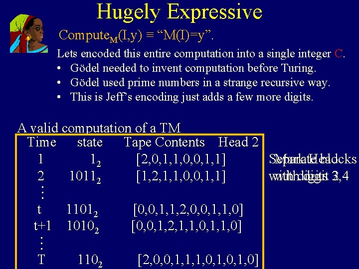
Hugely Expressive Compute. M(I, y) ≡ “M(I)=y”. Lets encoded this entire computation into a single integer C. • Gödel needed to invent computation before Turing. • Gödel used prime numbers in a strange recursive way. • This is Jeff’s encoding just adds a few more digits. … A valid computation of a TM Time state Tape Contents Head 2 1 12 [2, 0, 1, 1, 0, 0, 1, 1] Separate blocks Mark Head 2 10112 [1, 2, 1, 1, 0, 0, 1, 1] with digits 3, 4 with digit 2 … t 11012 [0, 0, 1, 1, 2, 0, 0, 1, 1, 0] t+1 10102 [0, 0, 1, 2, 1, 1, 0] T 1102 [2, 0, 0, 1, 1, 1, 0, 1, 0]

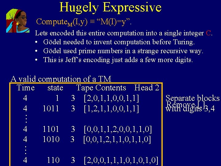
Hugely Expressive Compute. M(I, y) ≡ “M(I)=y”. Lets encoded this entire computation into a single integer C. • Gödel needed to invent computation before Turing. • Gödel used prime numbers in a strange recursive way. • This is Jeff’s encoding just adds a few more digits. … A valid computation of a TM Time state Tape Contents Head 2 4 1 3 [2, 0, 1, 1, 0, 0, 1, 1] Separate blocks Remove [, ] 4 1011 3 [1, 2, 1, 1, 0, 0, 1, 1] with digits 3, 4 4 1101 3 [0, 0, 1, 1, 2, 0, 0, 1, 1, 0] 4 1010 3 [0, 0, 1, 2, 1, 1, 0] … 4 110 3 [2, 0, 0, 1, 1, 1, 0, 1, 0]

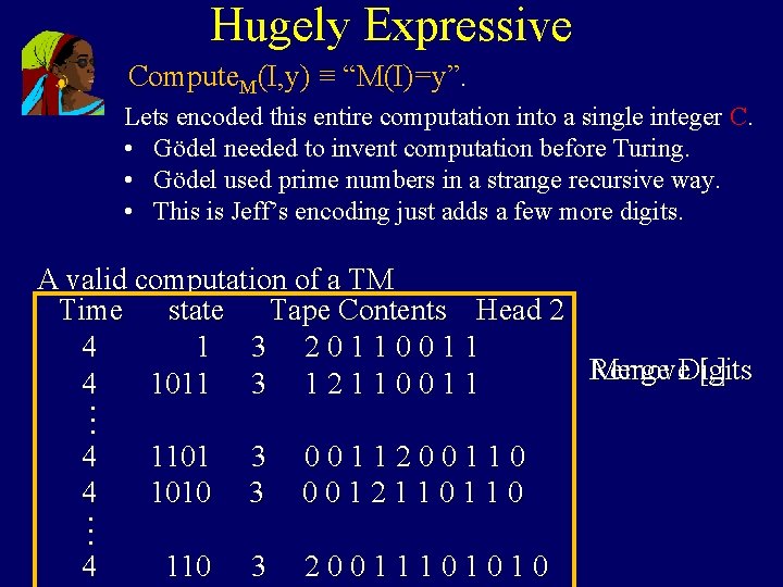
Hugely Expressive Compute. M(I, y) ≡ “M(I)=y”. Lets encoded this entire computation into a single integer C. • Gödel needed to invent computation before Turing. • Gödel used prime numbers in a strange recursive way. • This is Jeff’s encoding just adds a few more digits. … A valid computation of a TM Time state Tape Contents Head 2 4 1 3 2 0 1 1 0 0 1 1 Remove [, ] Merge Digits 4 1011 3 1 2 1 1 0 0 1 1 4 1101 3 0 0 1 1 2 0 0 1 1 0 4 1010 3 0 0 1 2 1 1 0 … 4 110 3 2 0 0 1 1 1 0 1 0

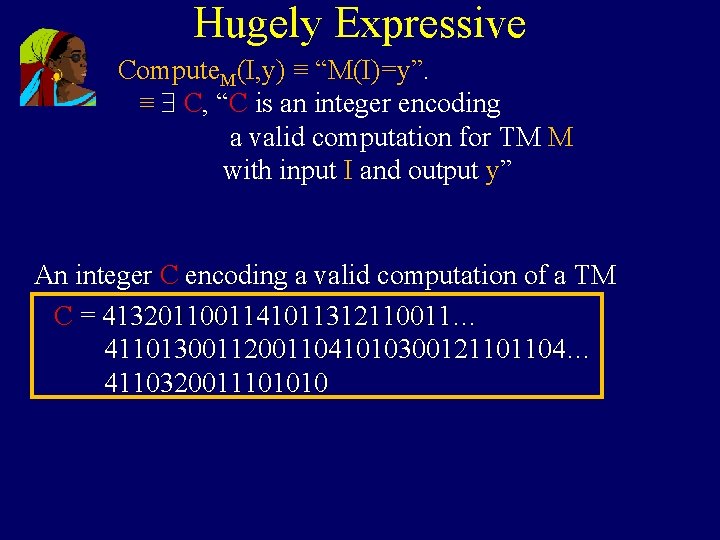
Hugely Expressive Compute. M(I, y) ≡ “M(I)=y”. Lets encoded this entire computation into a single integer C. • Gödel needed to invent computation before Turing. • Gödel used prime numbers in a strange recursive way. • This is Jeff’s encoding just adds a few more digits. An integer C encoding a valid computation of a TM C = 4132011001141011312110011… 411013001120011041010300121101104… 4110320011101010

Hugely Expressive Compute. M(I, y) ≡ “M(I)=y”. ≡ C, “C is an integer encoding a valid computation for TM M with input I and output y” An integer C encoding a valid computation of a TM C = 4132011001141011312110011… 411013001120011041010300121101104… 4110320011101010

Hugely Expressive “The initial config is that for TM M on input I” “C is an integer encoding “time t” “a legal TM ≡ a valid comp for TM M M step is taken” with input I and output y” “The final config is halting with y on tape” An integer C encoding a valid computation of a TM C = 4132011001141011312110011… 411013001120011041010300121101104… 4110320011101010

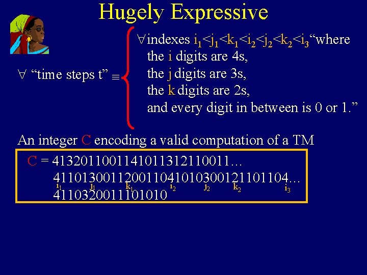
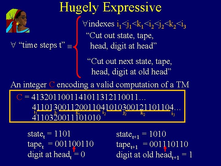
Hugely Expressive “time steps t” ≡ indexes i 1<j 1<k 1<i 2<j 2<k 2<i 3“where the i digits are 4 s, the j digits are 3 s, the k digits are 2 s, and every digit in between is 0 or 1. ” An integer C encoding a valid computation of a TM C = 4132011001141011312110011… 411013001120011041010300121101104… i 1 j 1 i 2 j 2 k 1 k 2 i 3 4110320011101010

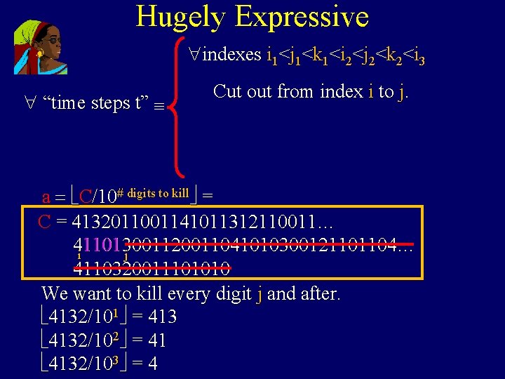
Hugely Expressive indexes i 1<j 1<k 1<i 2<j 2<k 2<i 3 “time steps t” ≡ Cut out from index i to j. a = C/10# digits to kill = C = 4132011001141011312110011… 1101 j 411013001120011041010300121101104… i 4110320011101010 We want to kill every digit j and after. 4132/101 = 4132/102 = 41 4132/103 = 4

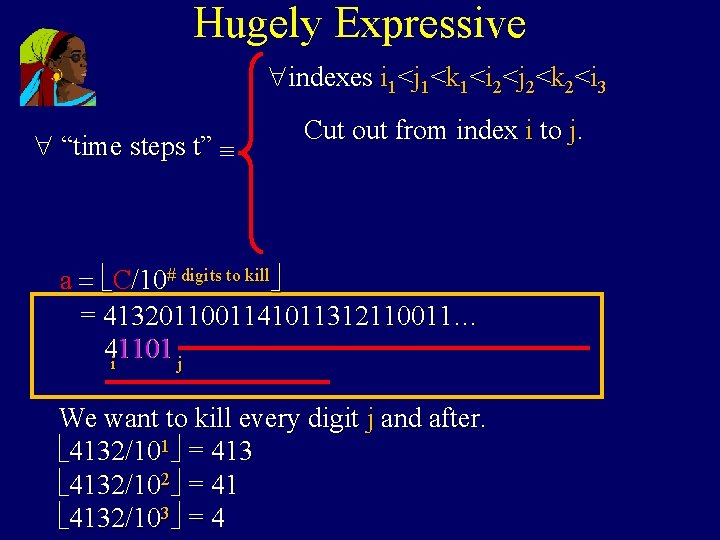
Hugely Expressive indexes i 1<j 1<k 1<i 2<j 2<k 2<i 3 “time steps t” ≡ Cut out from index i to j. a = C/10# digits to kill = 4132011001141011312110011… 1101 j 41101 i We want to kill every digit j and after. 4132/101 = 4132/102 = 41 4132/103 = 4

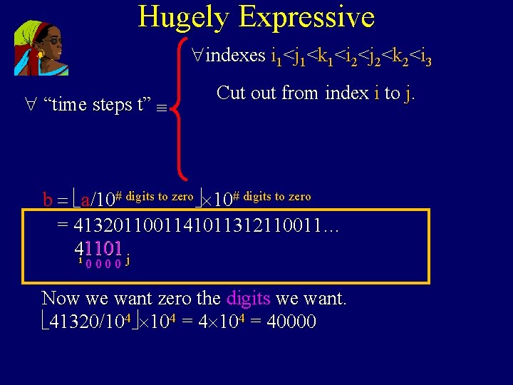
Hugely Expressive indexes i 1<j 1<k 1<i 2<j 2<k 2<i 3 “time steps t” ≡ Cut out from index i to j. b = a/10# digits to zero = 4132011001141011312110011… 1101 41101 i 0 0 j Now we want zero the digits we want. 41320/104 = 4 4 104 = 40000

Hugely Expressive indexes i 1<j 1<k 1<i 2<j 2<k 2<i 3 “time steps t” ≡ Cut out from index i to j. b = a/10# digits to zero = 4132011001141011312110011… 4 i 0000 j 0 0 Now we want zero the digits we want. 41320/104 = 4 4 104 = 40000

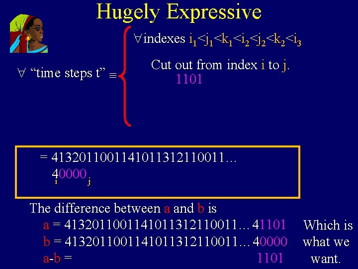
Hugely Expressive indexes i 1<j 1<k 1<i 2<j 2<k 2<i 3 “time steps t” ≡ Cut out from index i to j. 1101 = 4132011001141011312110011… 4 i 0000 j The difference between a and b is a = 4132011001141011312110011… 41101 Which is b = 4132011001141011312110011… 40000 what we a-b = 1101 want.

Hugely Expressive “time steps t” ≡ indexes i 1<j 1<k 1<i 2<j 2<k 2<i 3 “Cut out state, tape, head, digit at head” “Cut out next state, tape, head, digit at old head” An integer C encoding a valid computation of a TM C = 4132011001141011312110011… 411013001120011041010300121101104… i 1 j 1 i 2 j 2 k 1 k 2 i 3 4110320011101010 statet = 1101 tapet = 00110 digit at headt = 0 statet+1 = 1010 tapet+1 = 001110110 digit at old headt+1 = 1

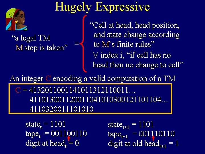
Hugely Expressive “a legal TM ≡ M step is taken” “Cell at head, head position, and state change according to M’s finite rules” index i, “if cell has no head then no change to cell” An integer C encoding a valid computation of a TM C = 4132011001141011312110011… 411013001120011041010300121101104… 4110320011101010 statet = 1101 tapet = 00110 digit at headt = 0 statet+1 = 1101 tapet+1 = 001110110 digit at old headt+1 = 1

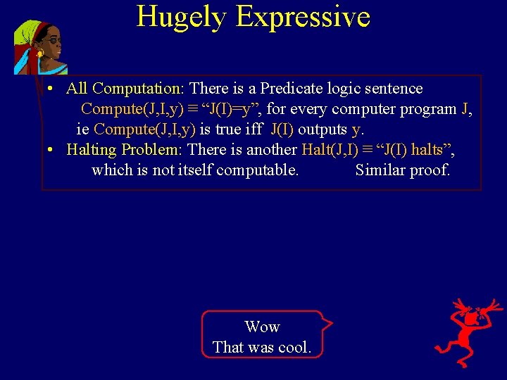
Hugely Expressive • All Computation: There is a Predicate logic sentence Compute(J, I, y) ≡ “J(I)=y”, for every computer program J, ie Compute(J, I, y) is true iff J(I) outputs y. • Halting Problem: There is another Halt(J, I) ≡ “J(I) halts”, which is not itself computable. Similar proof. Wow That was cool.

End