Logic and Computer Design Fundamentals Chapter 5 Sequential

Logic and Computer Design Fundamentals Chapter 5 – Sequential Circuits Part 2 – Sequential Circuit Design Charles Kime & Thomas Kaminski © 2008 Pearson Education, Inc. (Hyperlinks are active in View Show mode)

Overview § Part 1 - Storage Elements and Sequential Circuit Analysis § Part 2 - Sequential Circuit Design § Specification § Formulation § State Assignment § Flip-Flop Input and Output Equation Determination § Verification Chapter 5 - Part 2 2

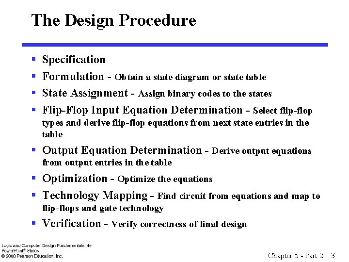
The Design Procedure § § Specification Formulation - Obtain a state diagram or state table State Assignment - Assign binary codes to the states Flip-Flop Input Equation Determination - Select flip-flop types and derive flip-flop equations from next state entries in the table § Output Equation Determination - Derive output equations from output entries in the table § Optimization - Optimize the equations § Technology Mapping - Find circuit from equations and map to flip-flops and gate technology § Verification - Verify correctness of final design Chapter 5 - Part 2 3

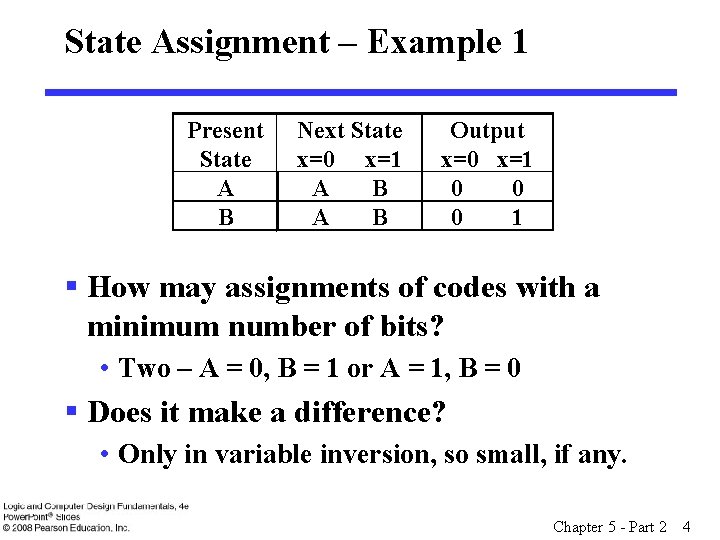
State Assignment – Example 1 Present State A B Next State x=0 x=1 A B Output x=0 x=1 0 0 0 1 § How may assignments of codes with a minimum number of bits? • Two – A = 0, B = 1 or A = 1, B = 0 § Does it make a difference? • Only in variable inversion, so small, if any. Chapter 5 - Part 2 4

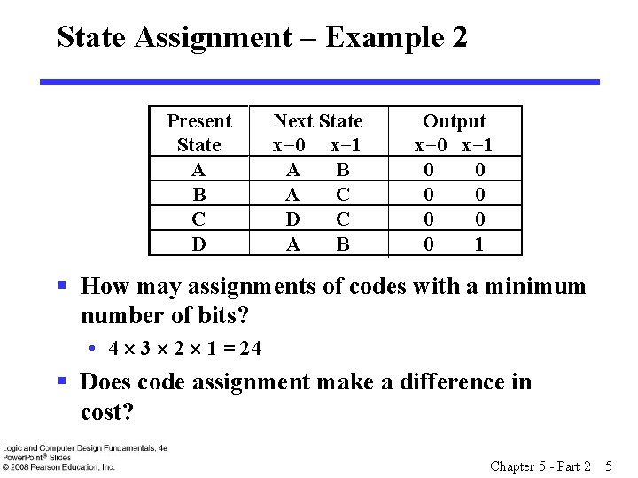
State Assignment – Example 2 Present State A B C D Next State x=0 x=1 A B A C D C A B Output x=0 x=1 0 0 0 0 1 § How may assignments of codes with a minimum number of bits? • 4 3 2 1 = 24 § Does code assignment make a difference in cost? Chapter 5 - Part 2 5

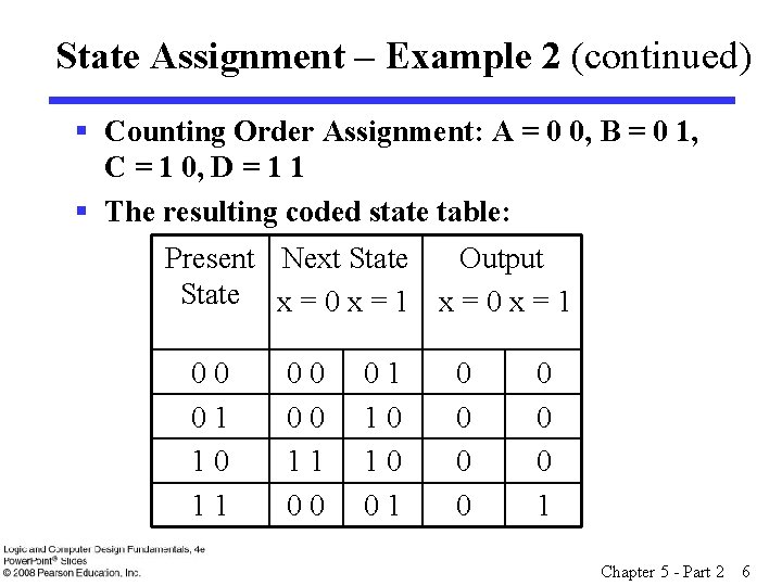
State Assignment – Example 2 (continued) § Counting Order Assignment: A = 0 0, B = 0 1, C = 1 0, D = 1 1 § The resulting coded state table: Present Next State Output State x = 0 x = 1 00 01 10 11 00 01 10 10 01 0 0 0 0 1 Chapter 5 - Part 2 6

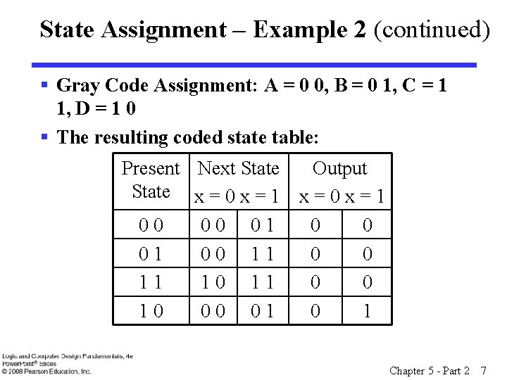
State Assignment – Example 2 (continued) § Gray Code Assignment: A = 0 0, B = 0 1, C = 1 1, D = 1 0 § The resulting coded state table: Present Next State Output State x = 0 x = 1 00 00 01 00 11 0 0 11 10 11 0 0 10 00 01 0 1 Chapter 5 - Part 2 7

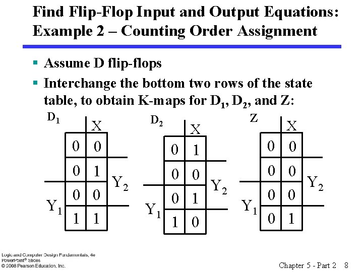
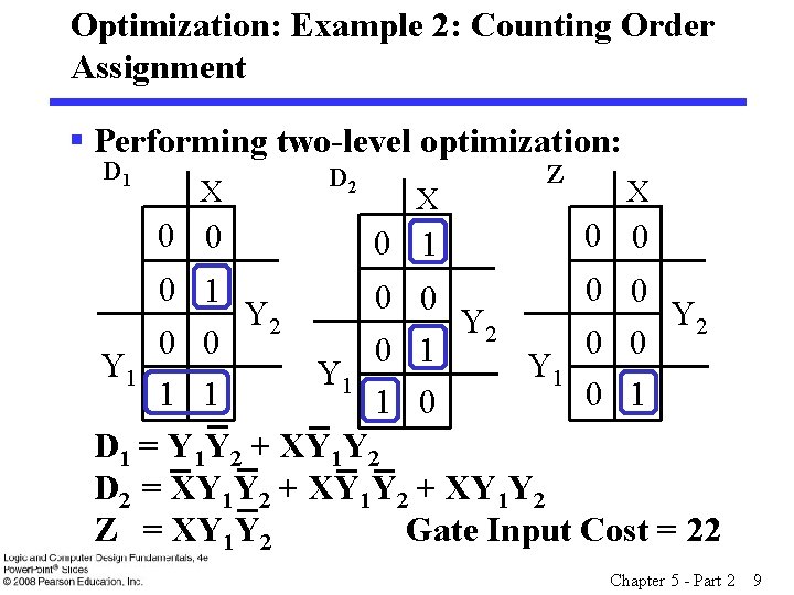
Find Flip-Flop Input and Output Equations: Example 2 – Counting Order Assignment § Assume D flip-flops § Interchange the bottom two rows of the state table, to obtain K-maps for D 1, D 2, and Z: D 1 X 0 0 0 1 Y 2 0 0 Y 1 1 1 D 2 X 0 1 Z X 0 0 0 Y 2 0 0 0 1 Y 1 0 1 1 0 Chapter 5 - Part 2 8

Optimization: Example 2: Counting Order Assignment § Performing two-level optimization: D 1 X 0 0 D 2 X 0 1 Z X 0 0 0 1 0 0 Y 2 Y 2 0 0 0 1 Y 1 Y 1 1 1 0 D 1 = Y 1 Y 2 + XY 1 Y 2 D 2 = XY 1 Y 2 + XY 1 Y 2 Z = XY 1 Y 2 Gate Input Cost = 22 Chapter 5 - Part 2 9

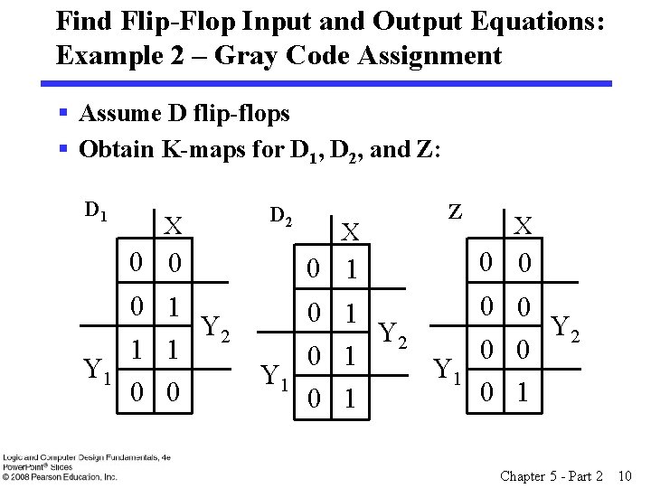
Find Flip-Flop Input and Output Equations: Example 2 – Gray Code Assignment § Assume D flip-flops § Obtain K-maps for D 1, D 2, and Z: D 1 X 0 0 0 1 Y 2 1 1 Y 1 0 0 D 2 X 0 1 Z X 0 0 0 1 Y 2 0 0 0 1 Y 1 0 1 Chapter 5 - Part 2 10

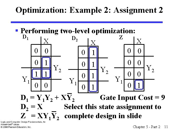
Optimization: Example 2: Assignment 2 § Performing two-level optimization: D 1 X 0 0 D 2 X 0 1 Z X 0 0 0 1 Y 2 1 1 Y 1 0 0 0 1 Y 2 0 0 0 1 Y 1 0 1 D 1 = Y 1 Y 2 + XY 2 Gate Input Cost = 9 D 2 = X Select this state assignment to Z = XY 1 Y 2 complete design in slide Chapter 5 - Part 2 11

One Flip-flop per State (One-Hot) Assignment § Example codes for four states: (Y 3, Y 2, Y 1, Y 0) = 0001, 0010, 0100, and 1000. § In equations, need to include only the variable that is 1 for the state, e. g. , state with code 0001, is represented in equations by Y 0 instead of Y 3 Y 2 Y 1 Y 0 because all codes with 0 or two or more 1 s have don’t care next state values. § Provides simplified analysis and design § Combinational logic may be simpler, but flipflop cost higher – may or may not be lower cost Chapter 5 - Part 2 12

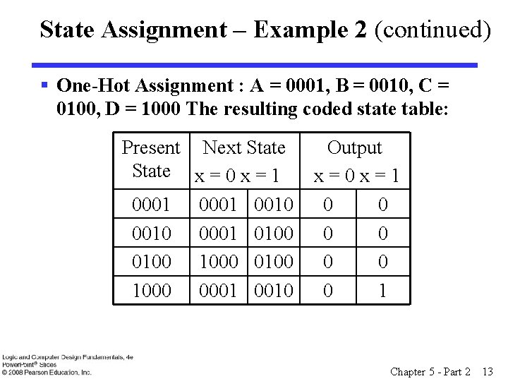
State Assignment – Example 2 (continued) § One-Hot Assignment : A = 0001, B = 0010, C = 0100, D = 1000 The resulting coded state table: Present Next State x = 0 x = 1 0001 0010 0001 0100 1000 0001 0010 Output x=0 x=1 0 0 0 0 1 Chapter 5 - Part 2 13

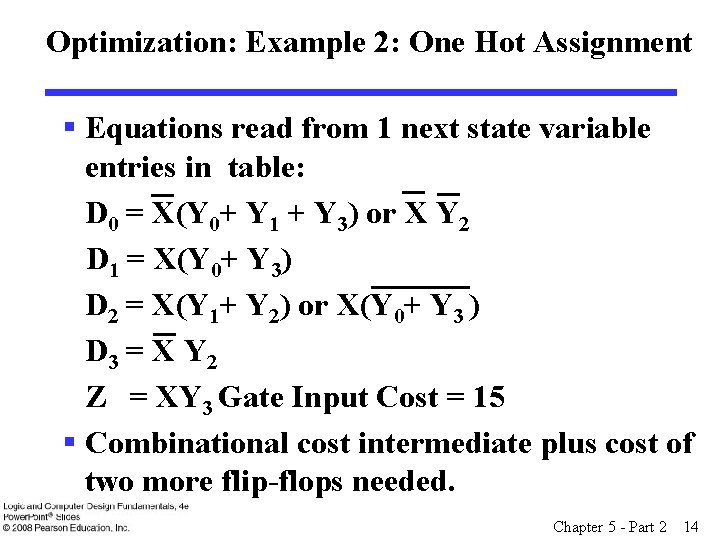
Optimization: Example 2: One Hot Assignment § Equations read from 1 next state variable entries in table: D 0 = X(Y 0+ Y 1 + Y 3) or X Y 2 D 1 = X(Y 0+ Y 3) D 2 = X(Y 1+ Y 2) or X(Y 0+ Y 3 ) D 3 = X Y 2 Z = XY 3 Gate Input Cost = 15 § Combinational cost intermediate plus cost of two more flip-flops needed. Chapter 5 - Part 2 14

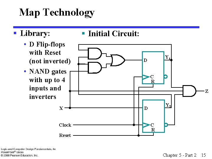
Map Technology § Library: § Initial Circuit: • D Flip-flops with Reset (not inverted) • NAND gates with up to 4 inputs and inverters X Clock Y 1 D C R Z Y 2 D C R Reset Chapter 5 - Part 2 15

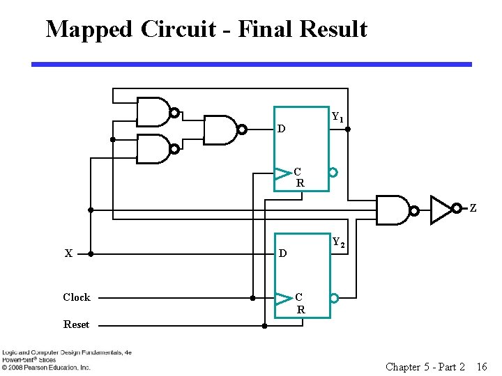
Mapped Circuit - Final Result Y 1 D C R Z X Clock Y 2 D C R Reset Chapter 5 - Part 2 16

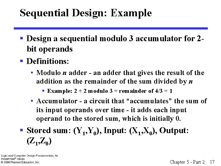
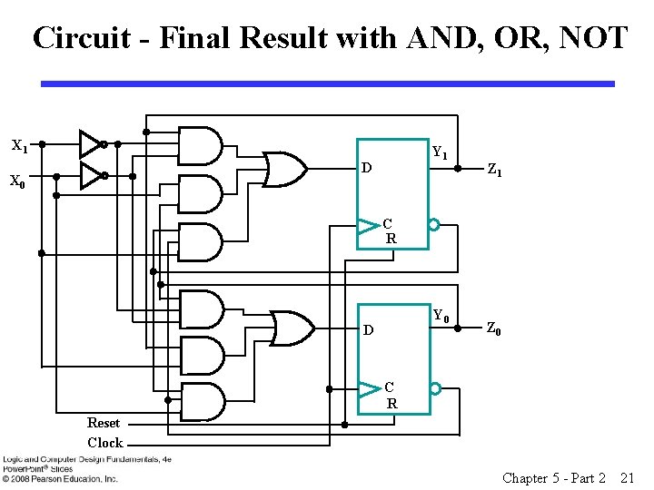
Sequential Design: Example § Design a sequential modulo 3 accumulator for 2 bit operands § Definitions: • Modulo n adder - an adder that gives the result of the addition as the remainder of the sum divided by n § Example: 2 + 2 modulo 3 = remainder of 4/3 = 1 • Accumulator - a circuit that “accumulates” the sum of its input operands over time - it adds each input operand to the stored sum, which is initially 0. § Stored sum: (Y 1, Y 0), Input: (X 1, X 0), Output: (Z 1, Z 0) Chapter 5 - Part 2 17

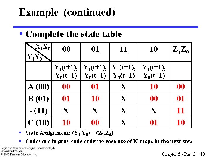
Example (continued) § Complete the state table X 1 X 0 Y 1 Y 0 00 01 11 10 Z 1 Z 0 Y 1(t+1), Y 0(t+1) A (00) B (01) - (11) C (10) 00 01 X 10 01 10 X 00 X X 10 00 X 01 00 01 11 10 § State Assignment: (Y 1, Y 0) = (Z 1, Z 0) § Codes are in gray code order to ease use of K-maps in the next step Chapter 5 - Part 2 18

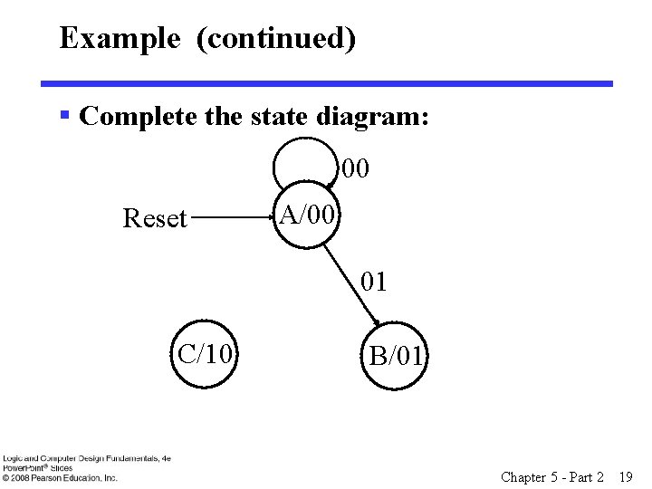
Example (continued) § Complete the state diagram: 00 Reset A/00 01 C/10 B/01 Chapter 5 - Part 2 19

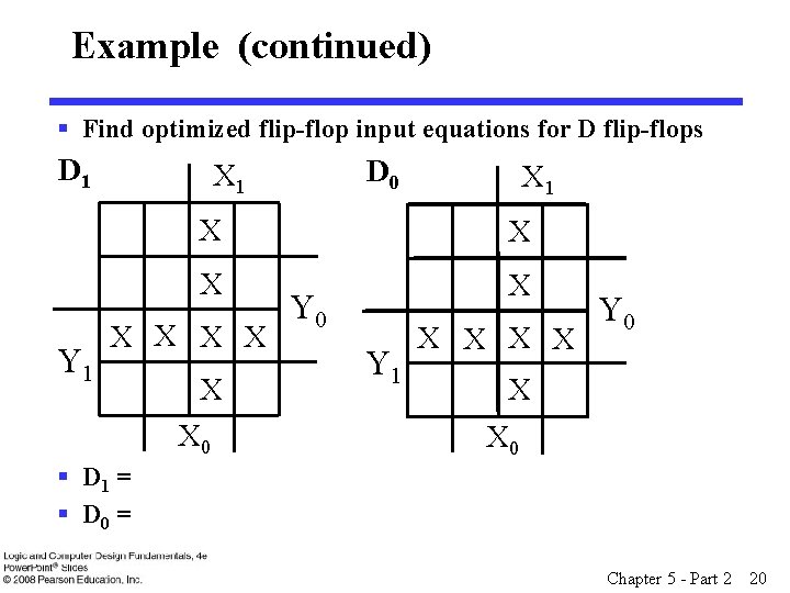
Example (continued) § Find optimized flip-flop input equations for D flip-flops D 1 Y 1 D 0 X 1 X X X X X 0 Y 1 X X Y 0 X X 0 § D 1 = § D 0 = Chapter 5 - Part 2 20

Circuit - Final Result with AND, OR, NOT X 1 Y 1 D X 0 Z 1 C R Y 0 D Z 0 C R Reset Clock Chapter 5 - Part 2 21

Other Flip-Flop Types § J-K and T flip-flops • Behavior • Implementation § Basic descriptors for understanding and using different flip-flop types • Characteristic tables • Characteristic equations • Excitation tables § For actual use, see Reading Supplement - Design and Analysis Using J-K and T Flip-Flops Chapter 5 - Part 2 22

J-K Flip-flop § Behavior • Same as S-R flip-flop with J analogous to S and K analogous to R • Except that J = K = 1 is allowed, and • For J = K = 1, the flip-flop changes to the opposite state • As a master-slave, has same “ 1 s catching” behavior as S-R flip-flop • If the master changes to the wrong state, that state will be passed to the slave § E. g. , if master falsely set by J = 1, K = 1 cannot reset it during the current clock cycle Chapter 5 - Part 2 23

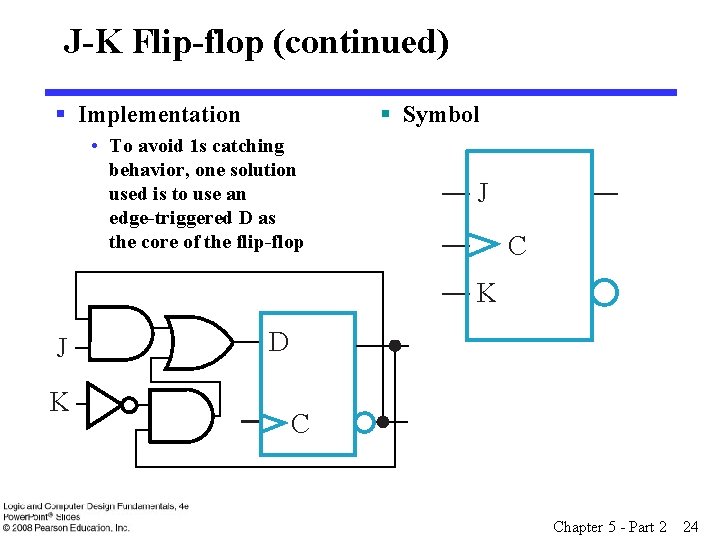
J-K Flip-flop (continued) § Implementation § Symbol • To avoid 1 s catching behavior, one solution used is to use an edge-triggered D as the core of the flip-flop J C K J K D C Chapter 5 - Part 2 24

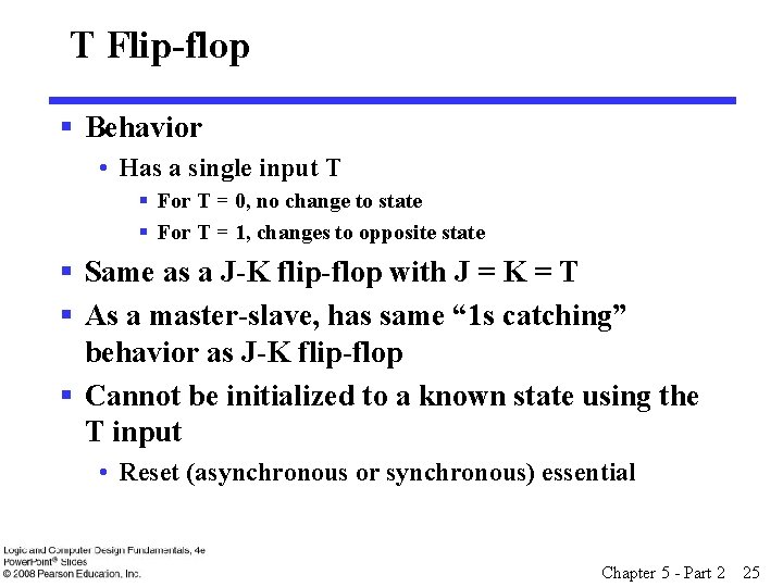
T Flip-flop § Behavior • Has a single input T § For T = 0, no change to state § For T = 1, changes to opposite state § Same as a J-K flip-flop with J = K = T § As a master-slave, has same “ 1 s catching” behavior as J-K flip-flop § Cannot be initialized to a known state using the T input • Reset (asynchronous or synchronous) essential Chapter 5 - Part 2 25

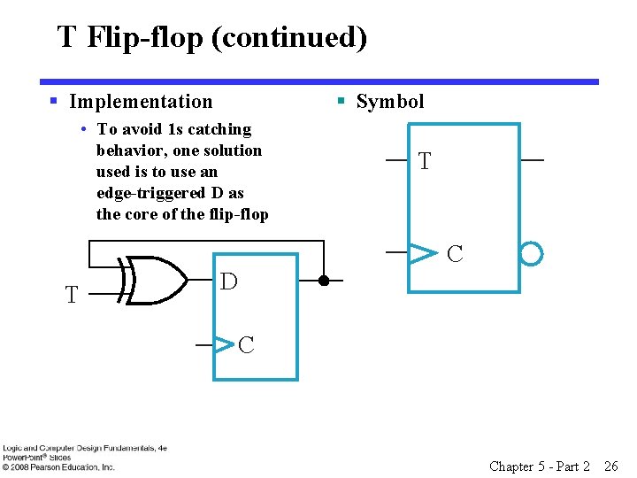
T Flip-flop (continued) § Implementation § Symbol • To avoid 1 s catching behavior, one solution used is to use an edge-triggered D as the core of the flip-flop T C T D C Chapter 5 - Part 2 26

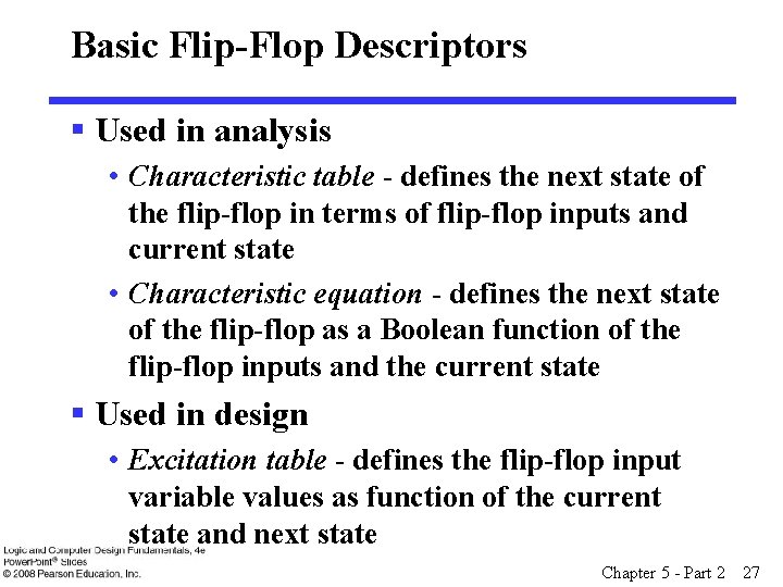
Basic Flip-Flop Descriptors § Used in analysis • Characteristic table - defines the next state of the flip-flop in terms of flip-flop inputs and current state • Characteristic equation - defines the next state of the flip-flop as a Boolean function of the flip-flop inputs and the current state § Used in design • Excitation table - defines the flip-flop input variable values as function of the current state and next state Chapter 5 - Part 2 27

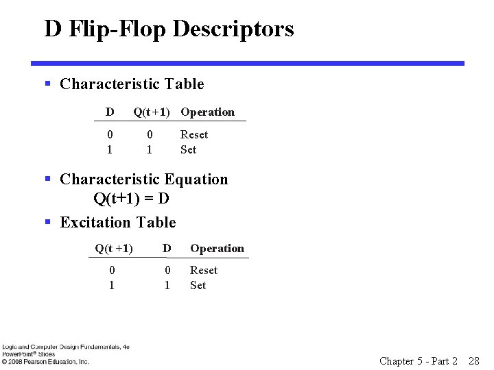
D Flip-Flop Descriptors § Characteristic Table D Q(t + 1) Operation 0 1 Reset Set § Characteristic Equation Q(t+1) = D § Excitation Table Q(t +1) D Operation 0 1 Reset Set Chapter 5 - Part 2 28

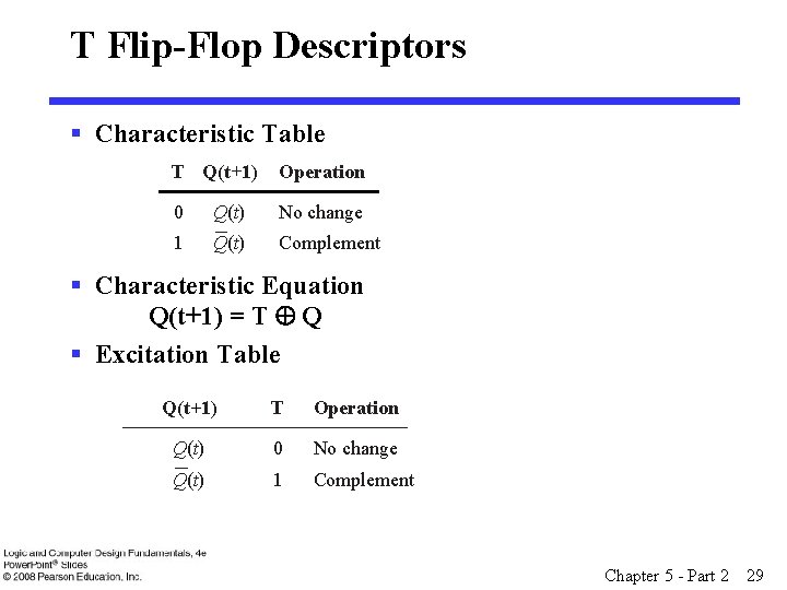
T Flip-Flop Descriptors § Characteristic Table T Q(t +1) Operation 0 Q(t) No change 1 Q(t) Complement § Characteristic Equation Q(t+1) = T Å Q § Excitation Table Q(t +1) T Operation Q(t) 0 No change Q(t) 1 Complement Chapter 5 - Part 2 29

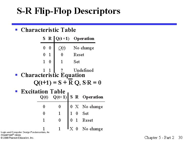
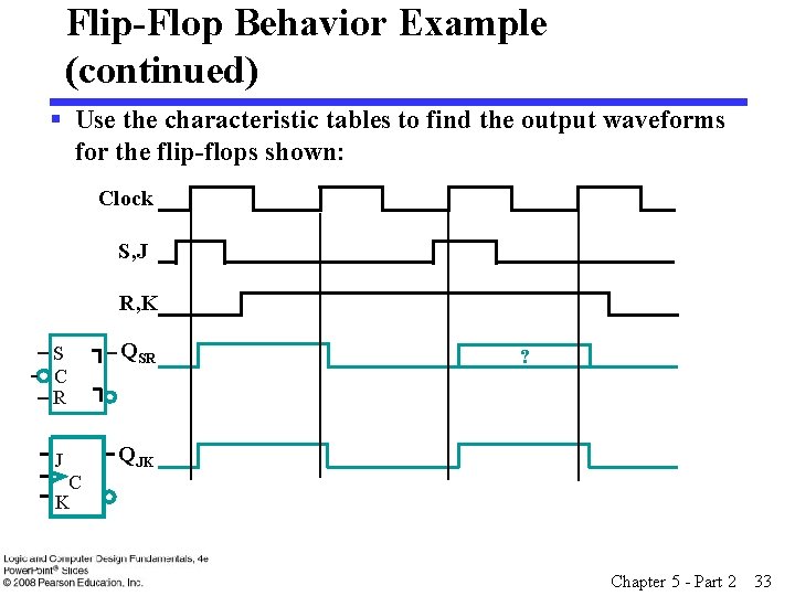
S-R Flip-Flop Descriptors § Characteristic Table S R Q(t +1) Operation 0 0 0 1 1 0 Q(t) 0 1 No change Reset Set 1 1 ? Undefined § Characteristic Equation Q(t+1) = S + R Q, S. R = 0 § Excitation Table Q(t) Q(t+ 1) S R Operation 0 0 1 0 0 X No change 1 0 Set 0 1 Reset 1 1 X 0 No change Chapter 5 - Part 2 30

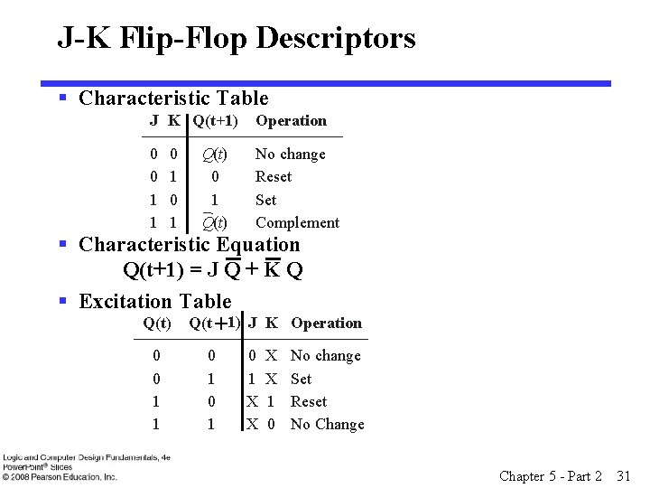
J-K Flip-Flop Descriptors § Characteristic Table J K Q(t+1) Operation 0 0 1 1 No change Reset Set Complement 0 1 Q(t) § Characteristic Equation Q(t+1) = J Q + K Q § Excitation Table Q(t) Q(t +1) J K Operation 0 0 1 1 0 1 0 1 X X 1 0 No change Set Reset No Change Chapter 5 - Part 2 31

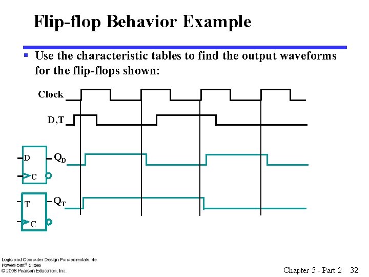
Flip-flop Behavior Example § Use the characteristic tables to find the output waveforms for the flip-flops shown: Clock D, T QD D C QT T C Chapter 5 - Part 2 32

Flip-Flop Behavior Example (continued) § Use the characteristic tables to find the output waveforms for the flip-flops shown: Clock S, J R, K S C R QSR J QJK ? C K Chapter 5 - Part 2 33