Location selection The selection of location is a

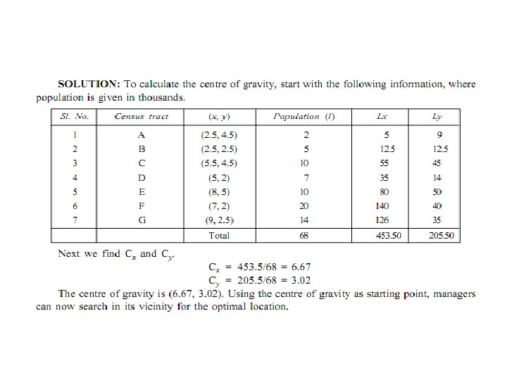
Location selection The selection of location is a key-decision as large investment is made in building plant and machinery. It is not advisable or not possible to change the location very often. So an improper location of plant may lead to waste of all the investments made in building and machinery, equipment. The plant location should be based on the company’s expansion plan and policy, diversification plan for the products, changing market conditions, the changing sources of raw materials and many other factors that influence the choice of the location decision.

FACTORS INFLUENCING PLANT LOCATION/FACILITY LOCATION It is appropriate to divide the factors, which influence the plant location or facility location on the basis of the nature of the organization as: 1. General locational factors, which include controllable and uncontrollable factors for all type of organizations. 2. Specific locational factors specifically required for manufacturing and service organizations.

General Locational Fcators

Controllable Factors: -Proximity to markets: -Supply of raw materials -transportation facilities -Infrastructure availability -labor and wages -external economies of scale -capital

• Proximity to markets: – • After sales services are promptly required very often. – • Transportation cost is high and increase the cost significantly. • Supply of raw materials • When a single raw material is used without loss of weight, • When raw material is universally available, locate close to the market area. • If the raw materials are processed from variety of locations, the plant may be situated • so as to minimize total transportation costs.

• 3. Transportation facilities: Speedy transport facilities ensure timely supply of raw materials to the company and finished goods to the customers. The transport facility is a prerequisite for • 4. Infrastructure availability: The basic infrastructure facilities like power, water and • waste disposal, etc. , become the prominent factors in deciding the location.

• Uncontrollable Factors: – Government policy – Climate condition – Supporting industries and services – Community and labor attitude – Community infrastructure and amenity(facility)

Specific locational factors for manufacturing organization Dominant factors: Location decisions for new manufacturing plants can be broadly classified in six groups. 1. favourable labor climate: labor-intensive firms in industries such as textiles, furniture, and consumer electronics. 2. Proximity to markets : For example, manufacturers of products such as plastic pipe and heavy metals all emphasize proximity to their markets. 3. Quality of life : Good schools, recreational facilities, cultural events, and an attractive lifestyle contribute to quality of life. 4. Proximity to suppliers and resources : 5. Utilities, taxes and real estate costs : telephone, energy, and water), – Secondary factors: room for expansion, construction costs, accessibility to multiple modes of transportation, the cost of shuffling people and materials between plants,

Specific locational factors for service organization Dominant factors 1. Proximity to customers : Example: few people would like to go to remotely located dry cleaner or supermarket if another is more convenient. 2. Transportation costs and proximity to markets : 3. Location of competitors : • Secondary factors: Retailers also must consider the level of retail activity, residential density, traffic flow, and site visibility. High residential density ensures nighttime and weekend business when the population in the area fits the firm’s competitive priorities and target market segment.

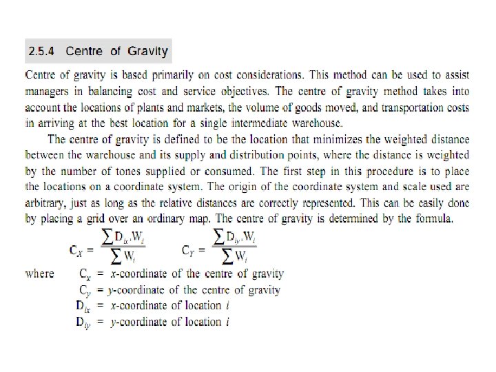
• Location models 1. 2. 3. 4. Weighted factor rating method Load-distance method Centre of gravity method Break even analysis

Weighted Factor Rating Method • In this method to merge quantitative and qualitative factors, factors are assigned weights based on relative importance and weightage score for each site using a preference matrix is calculated. The site with the highest weighted score is selected as the best choice.

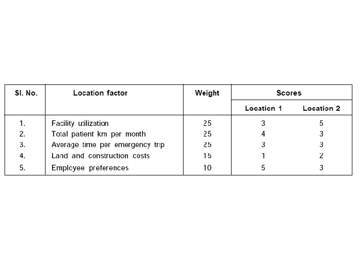
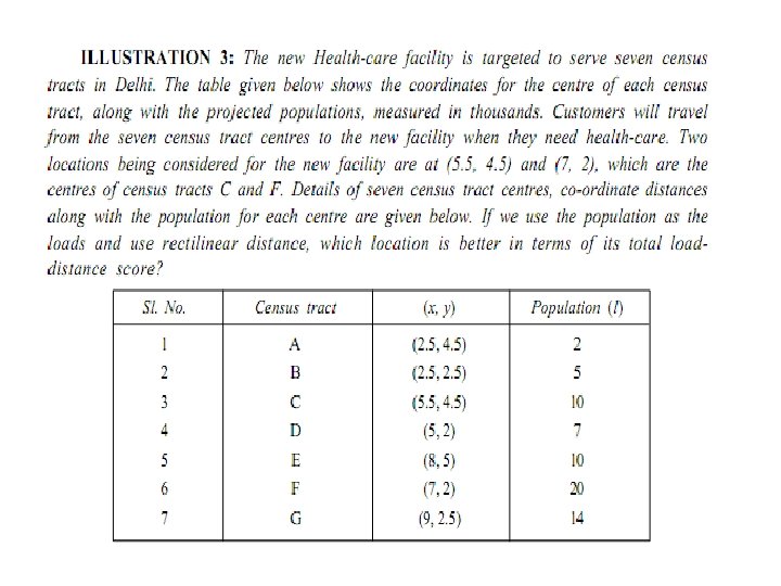
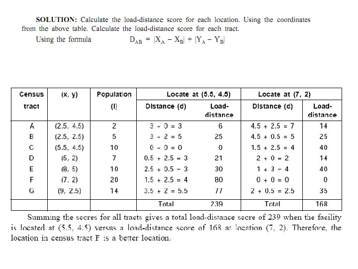
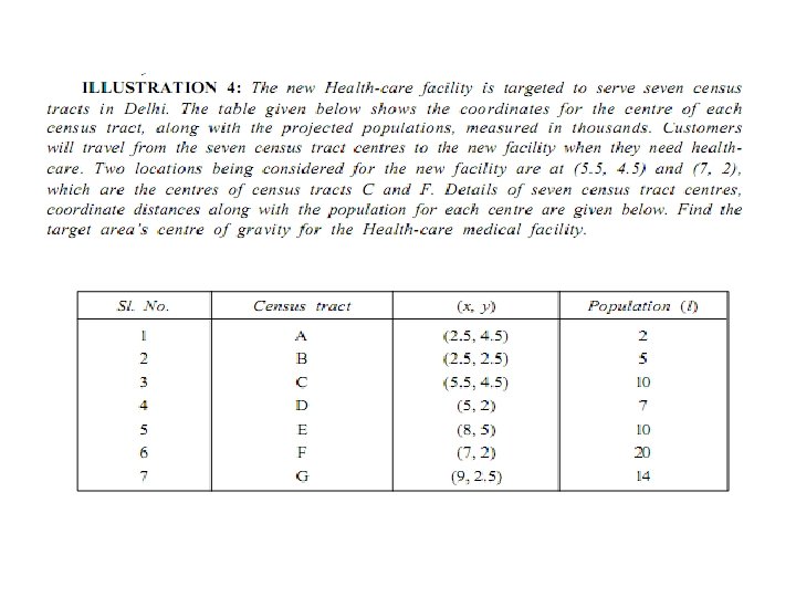
Problem • Let us assume that a new medical facility, Health-care, is to be located in Delhi. The location factors, weights, and scores (1 = poor, 5 = excellent) for two potential sites are shown in the following table. What is the weighted score for these sites? Which is the best location?

Solution • The weighted score for this particular site is calculated by multiplying each factor’s weight by its score and adding the results:

Application 11. 1 WS =

Revisiting Distance Measures What is the distance between (20, 10) and (80, 60)? Euclidean Distance d. AB = (20 – 80)2 + (10 – 60)2 = 78. 1 Rectilinear Distance d. AB = |20 – 80| + |10 – 60| = 110

Location North 200 y (miles) 150 Erie A (50, 185) 100 Pittsburgh 50 0 Uniontown 50 100 Scranton State College B (175, 100) Harrisburg Philadelphia 150 200 x (miles) 250 300 East

Location Euclidean distance d. AB = ( x. A – x. B )2 + ( y. A – y. B )2 (50 – 175 )2 + (185 – 100 )2 d. AB = 151. 2 miles

Location Rectilinear distance d. AB = | x. A – x. B | + | y. A – y. B | d. AB = | 50 – 175 | + | 185 – 100 | d. AB = 210 miles

Using OM Explorer Tutor 9. 2 - Distance Measures Enter the x and y coordinates of the two towns. Erie (Point A) State College (Point B) x 50 175 y 185 100 To find the Euclidian distance, subtract the second town’s x value from that of the first town, and square the result. Do the same with the two y values. Then add the two and compute the square root. (Erie x – State College x)2 (Erie y – State College y)2 15. 625 7, 225 Euclidian distance 151. 16 To find the rectilinear distance, get the absolute value of the result of subtracting the second town’s x from the first town’s. Do the same with y. Then add the absolute distances together. (Erie x – State College x) (Erie y – State College y) 125 85 Rectilinear distance 210

Using Break-Even Analysis • Break-even analysis can help a manager compare location alternatives on the basis of quantitative factors that can be expressed in terms of total cost. 1. Determine the variable costs and fixed costs for each site. 2. Plot the total cost lines—the sum of variable and fixed costs—for all the sites on a single graph 3. Identify the approximate ranges for which each location has the lowest cost. 4. Solve algebraically for the break-even points over the relevant ranges.

Break-Even Analysis Example 11. 4 • An operations manager has narrowed the search for a new facility location to four communities. • The annual fixed costs (land, property taxes, insurance, equipment, and buildings) and the variable costs (labor, materials, transportation, and variable overhead) are shown below. • Total costs are for 20, 000 units. Community Fixed Costs per Year Variable Costs per Unit Total Costs (Fixed + Variable) A B C D $150, 000 $300, 000 $500, 000 $62 $38 $24 $30 $1, 390, 000 $1, 060, 000 $ 980, 000 $1, 200, 000

Annual cost (thousands of dollars) ØStep 1. Plot the total cost curves for all the communities on a single graph. Identify on the graph the approximate range over which each community provides the lowest cost. Community Fixed Costs per Year Total Costs (Fixed + Variable) A B C D $150, 000 $300, 000 $500, 000 $600, 000 $1, 390, 000 $1, 060, 000 $ 980, 000 $1, 200, 000 1600 (20, 1390) 1400 (20, 1200) 1200 (20, 980) 800 Break-even point 600 Break-even point 400 200 0 © 2007 Pearson Education D B C (20, 1060) 1000 A best 2 4 B best 6 8 6. 25 C best 10 12 14 16 18 20 22 14. 3 Q (thousands of units) A

Comment: Figure shows the graph of the total cost lines. The line for community A goes from (0, 150) to (20, 1, 390). The graph indicates that community A is best for low volumes, B for intermediate volumes, and C for high volumes. We should no longer consider community D, because both its fixed and its variable cost are higher than community C’s.

Break-Even Solution Example 11. 4 • Step 2. Using break-even analysis, calculate the break-even quantities over the relevant ranges. If the expected demand is 15, 000 units per year, what is the best location? (A) (B) $150, 000 + $62 Q = $300, 000 + $38 Q Q = 6, 250 units (B) (C) $300, 000 + $38 Q = $500, 000 + $24 Q Q = 14, 286 units

Application 11. 5

Application 11. 5