Location planning and analysis Need for Location Decisions

Location planning and analysis

Need for Location Decisions • Marketing Strategy • Cost of Doing Business • Growth • Depletion of Resources

Nature of Location Decisions • Strategic Importance – – – Long term commitment/costs Impact on investments, revenues, and operations Supply chains • Objectives – – – Profit potential No single location may be better than others Identify several locations from which to choose • Options – – – Expand existing facilities Add new facilities Move

Making Location Decisions • • • Decide on the criteria Identify the important factors Develop location alternatives Evaluate the alternatives Make selection

Location Decision Factors Regional Factors Community Considerations Multiple Plant Strategies Site-related Factors

Regional Factors • • Location of raw materials Location of markets Labor factors Climate and taxes

Community Considerations • • Quality of life Services Attitudes Taxes Environmental regulations Utilities Developer support

Site Related Factors • • Land Transportation Environmental Legal

Multiple Plant Strategies • Product plant strategy • Market area plant strategy • Process plant strategy

Comparison of Service and Manufacturing Considerations Manufacturing/Distribution Service/Retail Cost Focus Revenue focus Transportation modes/costs Demographics: age, income, etc Energy availability, costs Population/drawing area Labor cost/availability/skills Competition Building/leasing costs Traffic volume/patterns Customer access/parking

Trends in Locations • Foreign producers locating in another country – – “Made in” effect Currency fluctuations • Just-in-time manufacturing techniques • Microfactories • Information Technology

3+1 methods to evaluate location alternatives • Locational Cost-Profit-Volume Analysis • Factor rating • The Center of Gravity method • The transportation model

Locational Cost-Profit-Volume Analysis • Numerical and graphical analysis are both feasible. We focus on the graphical one. • The steps: 1. Determine the fixed and variable costs for each location 2. Plot the total-cost lines for all location alternatives on the same graph 3. Determine which location will have the lowest total cost for the expected level of output. Alternatively, determine which location will have the highest profit.

Assumptions of the CPV Analysis • Fixed costs are constant for the range of probable output • Variable costs are linear for the range of probable output • The required level of output can be closely estimated • Only one product is involved

The total cost curve Cost • TC = FC + VC = FC + v*Q c l ta t s o To C V = le b ia s co t ) C (V r a lv ta o T C F + Fixed cost (FC) 0 Q (volume in units)

Alternatively, the total profit is • TP = Q * (R – v) – FC

A simple problem from the text-book Location Fixed cost (FC) Variable cost per unit (v) A 250, 000 11 B 100, 000 30 C 150, 000 20 D 200, 000 35

Plotting the total-cost lines

Calculate the break-even output levels • For B and C: 100, 000 + 30*Q = 150, 000 + 20*Q Q = 5, 000 • For C and A: 150, 000 + 20*Q = 250, 000 + 11*Q Q = 11, 111

Which location is the best? The expected long-term volume Best location > 11, 111 A 5, 000 < Exp. vol. < 11, 111 C < 5, 000 B

Another problem for the same method Location Fixed cost (FC) Variable cost per unit (v) A 10000 30 B 20000 20 C 35000 15 D 25000 40

The plot 120000 100000 80000 TC(A) TC(B) 60000 TC( C) TC(D) 40000 20000 0 1 2 3 4 5 6 7 8 9 10 11 12 13 14 15 16 17 18 19

Factor rating • Can be used for a wide range of problems • The procedure: – Determine the relevant factors – Assign a weight to each factor, indicating its importance (usually 0 -1) – Decide on a common scale of the factors and transform them to that scale – Score each location alternative – Multiply the factor weight by the score for each factor and sum the results for each location – Choose the alternative with the highest composite score

Example form the text-book

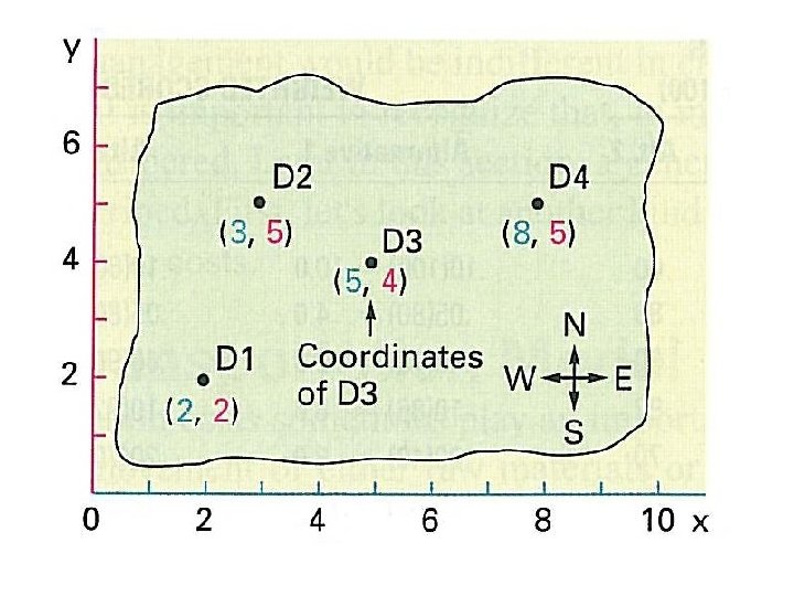
The Center of Gravity method • Its aim is to determine the location of a facility that will minimize the shipping cost or travel time to various destinations. • Frequently used in determining the location of schools, firefighter bases, public safety centres, highways, distribution centres, retail businesses…

Assumptions • The distribution cost is a linear function of the distance and the quantity shipped • The relative quantity shipped to each destination is fixed in time

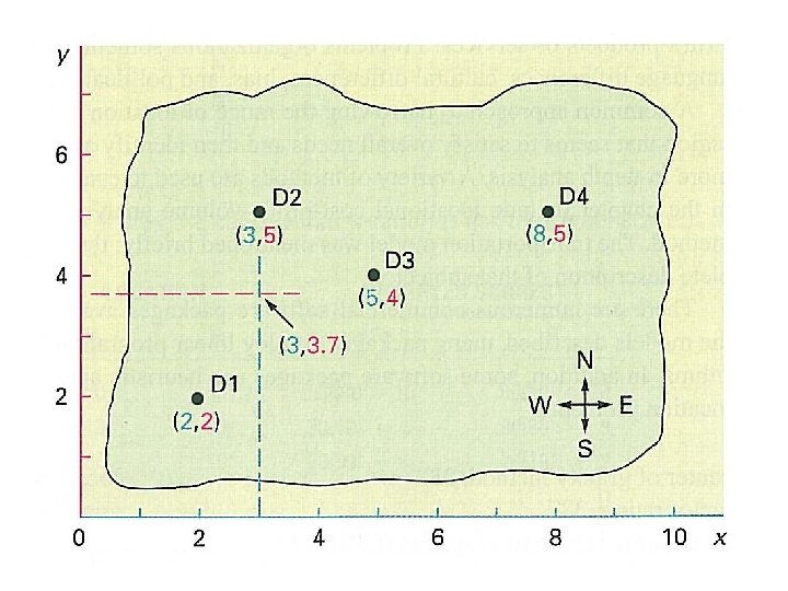
Map and coordinates • A map is needed that shows the locations of destinations • A coordinate system is overlaid on the map to determine the coordinates of each destination • The aim is to find the coordinates of the optimal location for the facility, as a weighted average of the x and y coordinates of each destinations, where the weights are the shipped quantities. This is the centre of gravity.

A sample problem

The formulas

The solution

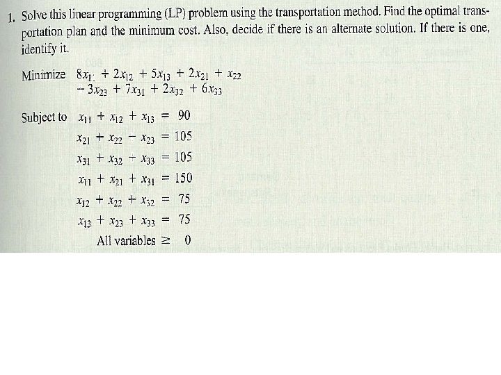
The transportation model A special case of the linear programming model

The transportation problem • …involves finding the lowest-cost plan for distributing stocks of supplies from multiple origins to multiple destinations that demand them.

The optimal shipping plan • The transportation model is used to determine how to allocate the supplies available at the origins to the customers, in such a way that total shipping cost is minimized. • The optimal set of shipments is called the optimal shipping plan. • There can be more optimal shipping plans. • The plan will change if any of the parameters changes significantly.

A possible transportation problem situation D D S S D

Defining the classic transportation problem • The goods have more shipping points (suppliers) and more destinations (buyers). • Prices are fixed. • The sum of the quantities supplied and the sum of quantities demanded are equal. There are no surpluses nor shortages. • ai and bj are both positive (there are no reverse flow of goods) • the dependent variables are the transported quantities form origin i to destination j: xij ≥ 0 • All of the supplies should be sold and all of the demand should be satisfied. • Tha aim is to minimize the total transportation cost: • Homogeneous goods. • Shipping costs per unit are constant. • Only one route and mode ofg transportation exists between each origin and each destination.

Typical areas of transportation problems • • Suppliers of components and assembly plants. Factories and shops. Suppliers of raw materials and factories. Food processing factories and food retailers.

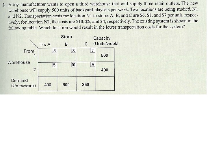
Informations needed to built a model • A list of the shipping points with their capacities (supply quantities). • A list of the destinations with their demand. • Transportation costs per unit from each origin to each destination • Question: what if prices of the good are differ form supplier to supplier?

Surplus • If the total supply is greater than the total demand, than we have to add a ‘phantom’ destination to the model the demand of which is equal to the surplus. • The transportation cost to this phantom destination is 0 from every supplier. • De quantities shipped to this virtual customer will be those that will not be bought by anybody.

Shortages • The formal solution is the same as it was in the case of a surplus (with 0 transportation costs): • But: mathematics are less adequate in the case of shortages than in the case of surplusses, because of the consequences.

The transportation table A B C D Supply 7 1 100 2 4 (unit 7 cost) 12 3 8 8 200 3 8 10 16 5 150 90 120 160 450= =450 1 Demand 80

Solving transportation problems • Never try without a computer • There can be many equivalent solutions (with the same total cost).

Creating models and solving them

Thanks for the attention!