Localization Navigation II Topological Representations What makes a

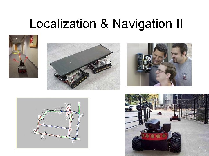
Localization & Navigation II

Topological Representations: What makes a good landmark? • Perceivable from many different viewpoints • Persistence • Distinct features – Readily recognizable • Unique features – Avoid sensor aliasing

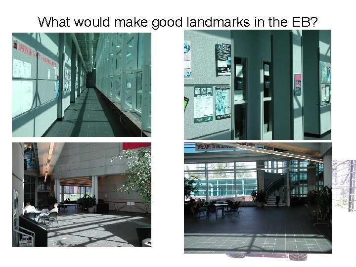
What would make good landmarks in the EB?

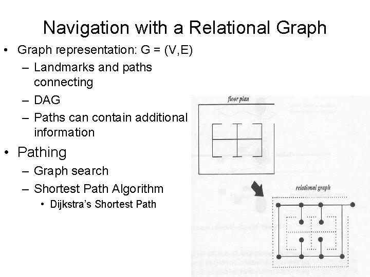
Navigation with a Relational Graph • Graph representation: G = (V, E) – Landmarks and paths connecting – DAG – Paths can contain additional information • Pathing – Graph search – Shortest Path Algorithm • Dijkstra’s Shortest Path

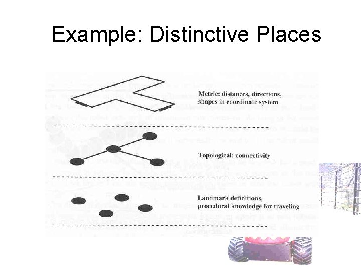
Example: Distinctive Places

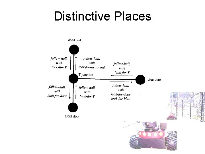
Distinctive Places

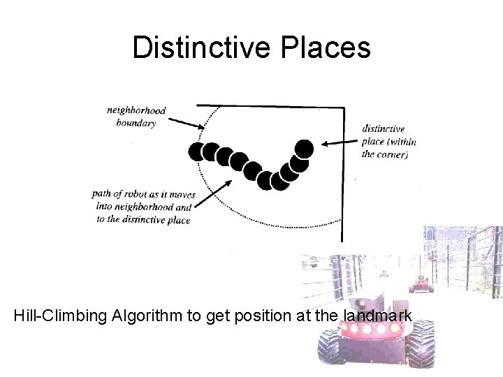
Distinctive Places Hill-Climbing Algorithm to get position at the landmark

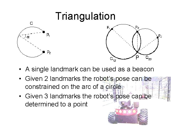
Triangulation • A single landmark can be used as a beacon • Given 2 landmarks the robot’s pose can be constrained on the arc of a circle • Given 3 landmarks the robot’s pose can be determined to a point

Metric Representations • Coordinate system representation • Path is decomposed into waypoints – As opposed to landmarks • Path planning is usually based on some measure of optimal or best path – Graph search or graph coloring methods

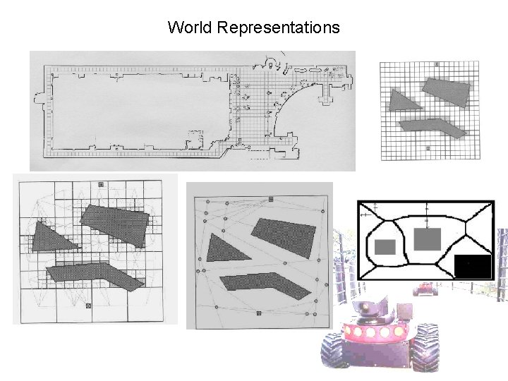
World Representations

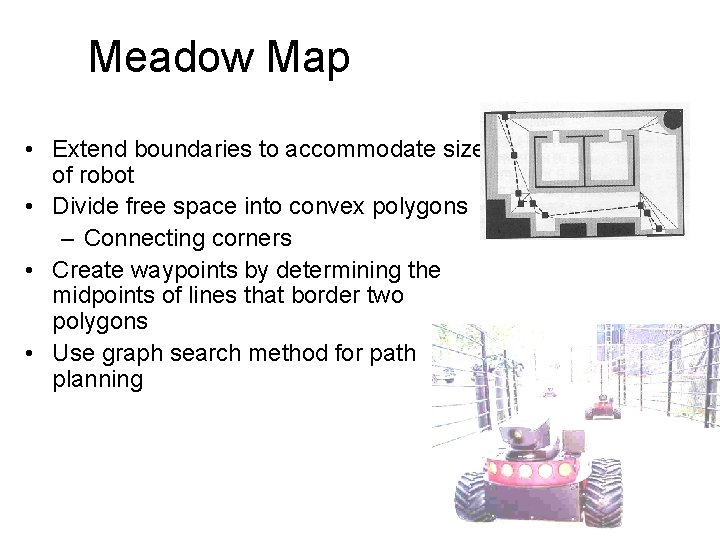
Meadow Map • Extend boundaries to accommodate size of robot • Divide free space into convex polygons – Connecting corners • Create waypoints by determining the midpoints of lines that border two polygons • Use graph search method for path planning

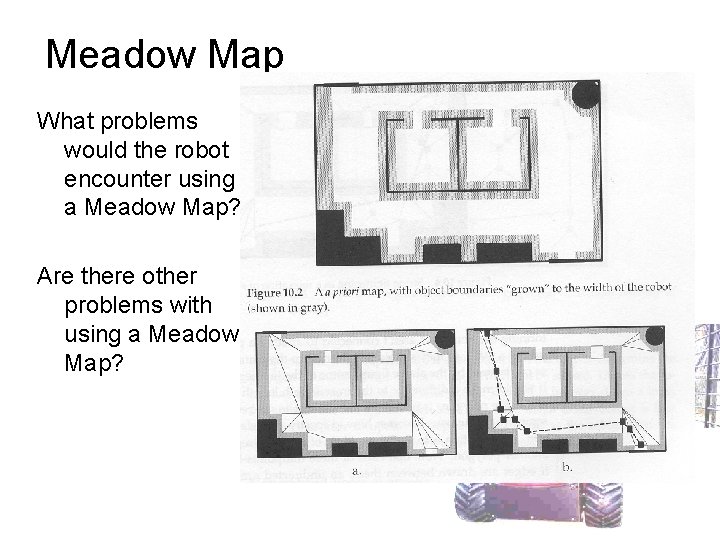
Meadow Map What problems would the robot encounter using a Meadow Map? Are there other problems with using a Meadow Map?

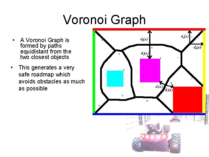
Voronoi Graph • A Voronoi Graph is formed by paths equidistant from the two closest objects • This generates a very safe roadmap which avoids obstacles as much as possible

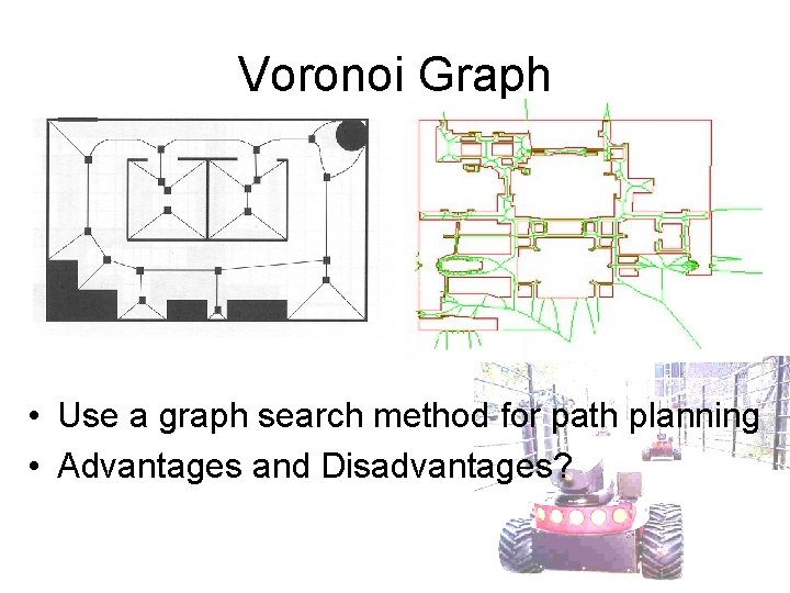
Voronoi Graph • Use a graph search method for path planning • Advantages and Disadvantages?

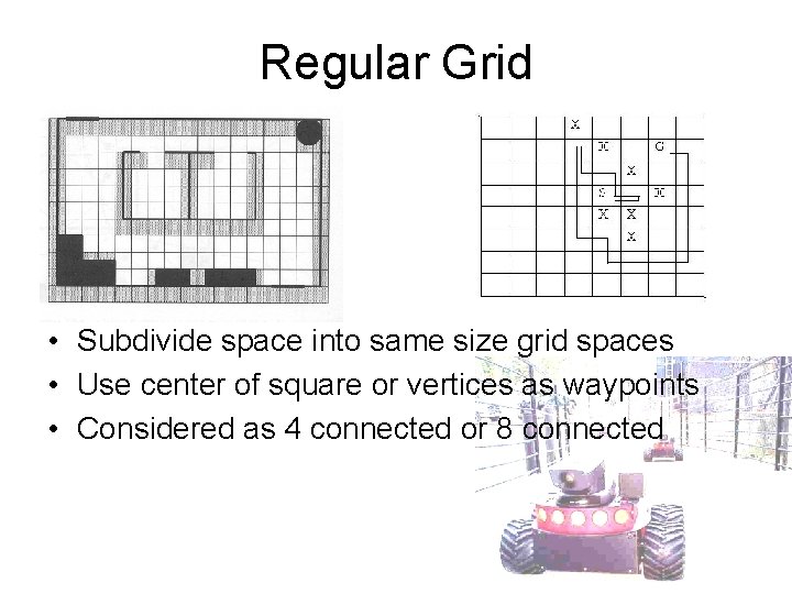
Regular Grid • Subdivide space into same size grid spaces • Use center of square or vertices as waypoints • Considered as 4 connected or 8 connected

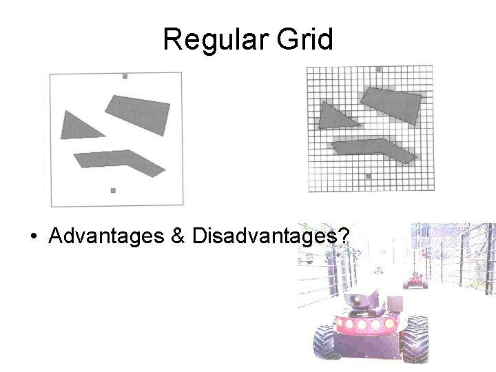
Regular Grid • Advantages & Disadvantages?

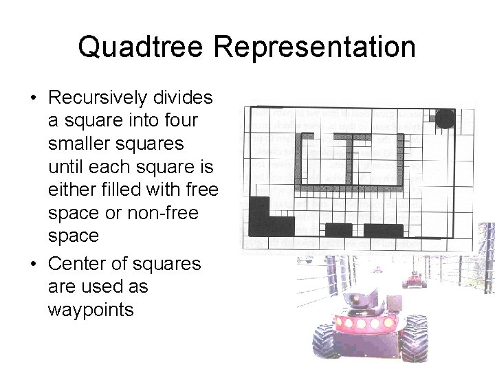
Quadtree Representation • Recursively divides a square into four smaller squares until each square is either filled with free space or non-free space • Center of squares are used as waypoints

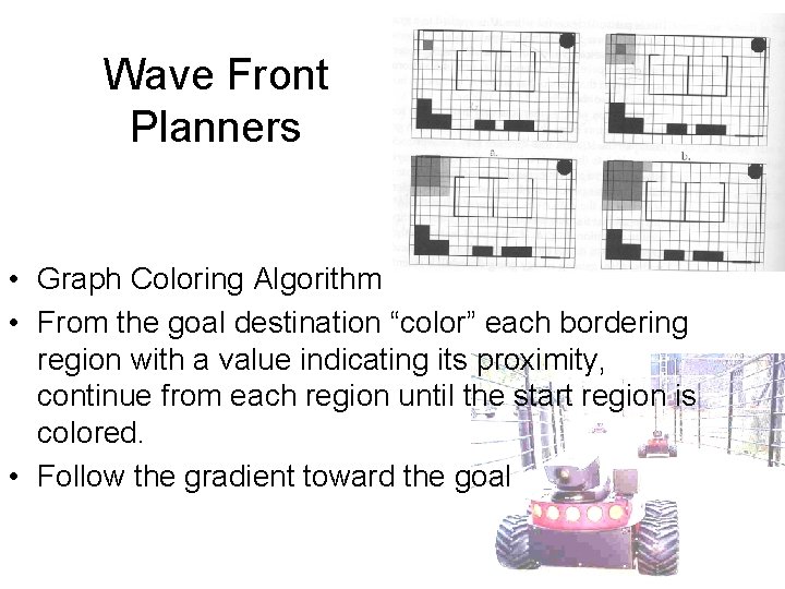
Wave Front Planners • Graph Coloring Algorithm • From the goal destination “color” each bordering region with a value indicating its proximity, continue from each region until the start region is colored. • Follow the gradient toward the goal

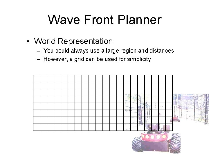
Wave Front Planner • World Representation – You could always use a large region and distances – However, a grid can be used for simplicity

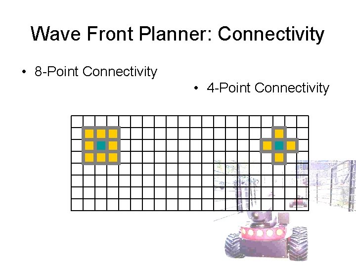
Wave Front Planner: Connectivity • 8 -Point Connectivity • 4 -Point Connectivity

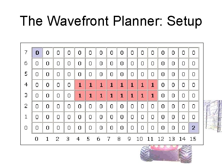
The Wavefront Planner: Setup

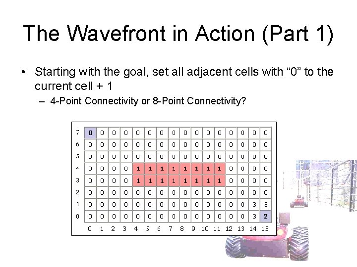
The Wavefront in Action (Part 1) • Starting with the goal, set all adjacent cells with “ 0” to the current cell + 1 – 4 -Point Connectivity or 8 -Point Connectivity?

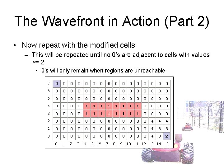
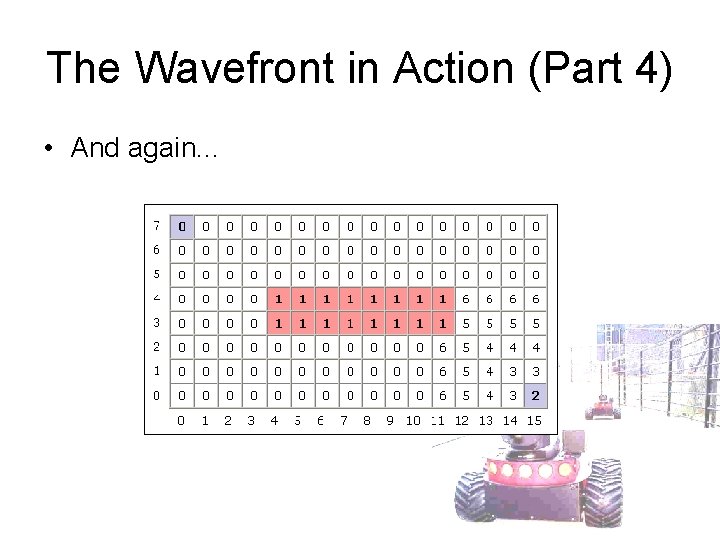
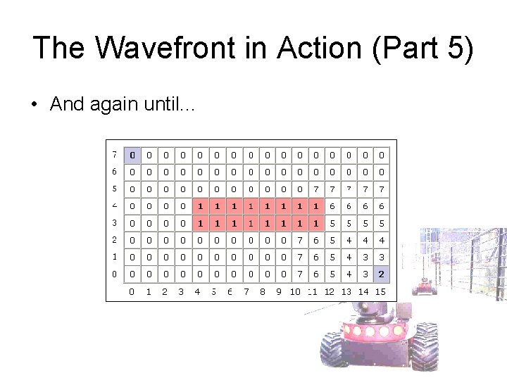
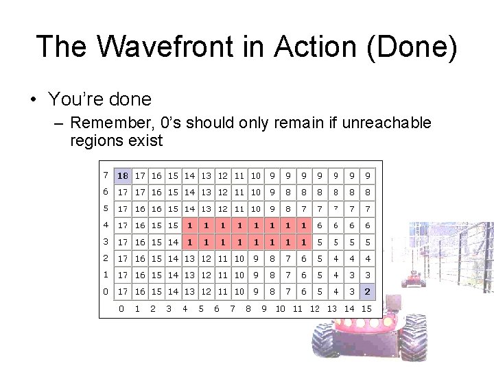
The Wavefront in Action (Part 2) • Now repeat with the modified cells – This will be repeated until no 0’s are adjacent to cells with values >= 2 • 0’s will only remain when regions are unreachable

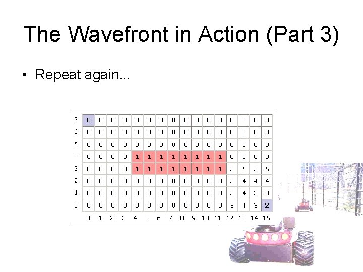
The Wavefront in Action (Part 3) • Repeat again. . .

The Wavefront in Action (Part 4) • And again. . .

The Wavefront in Action (Part 5) • And again until. . .

The Wavefront in Action (Done) • You’re done – Remember, 0’s should only remain if unreachable regions exist

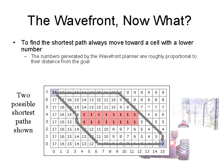
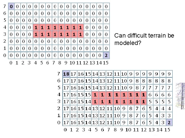
The Wavefront, Now What? • To find the shortest path always move toward a cell with a lower number – The numbers generated by the Wavefront planner are roughly proportional to their distance from the goal Two possible shortest paths shown

Can difficult terrain be modeled?

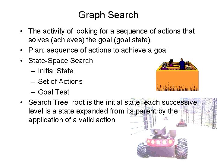
Graph Search • The activity of looking for a sequence of actions that solves (achieves) the goal (goal state) • Plan: sequence of actions to achieve a goal • State-Space Search – Initial State – Set of Actions – Goal Test • Search Tree: root is the initial state, each successive level is a state expanded from its parent by the application of a valid action

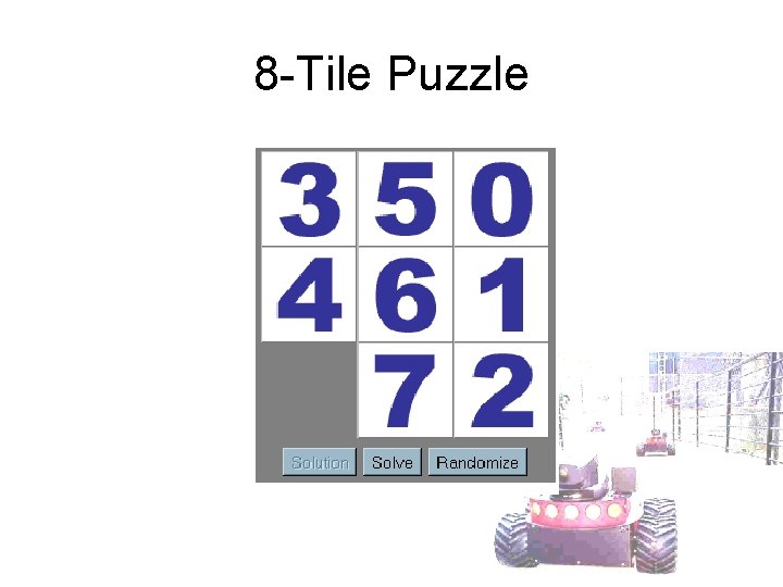
8 -Tile Puzzle

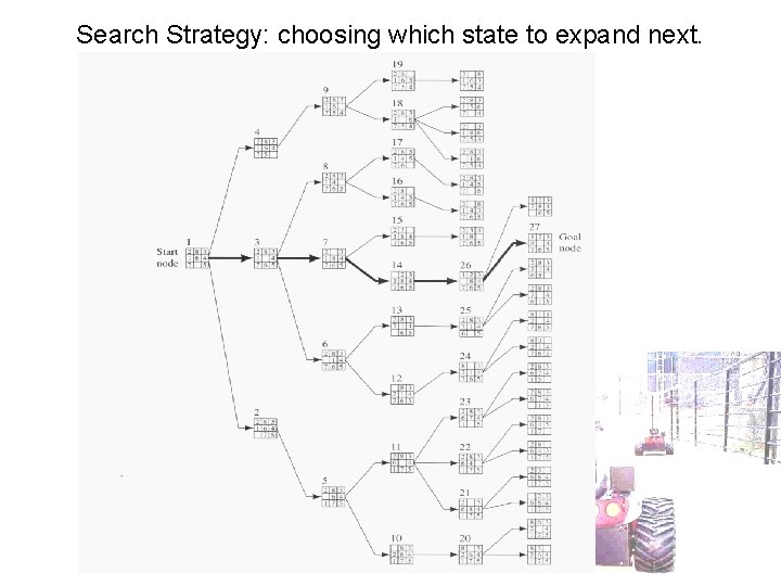
Search Strategy: choosing which state to expand next.

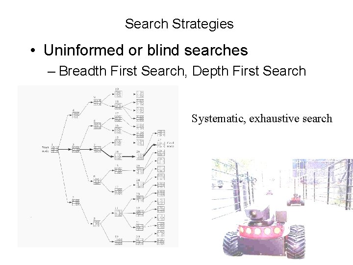
Search Strategies • Uninformed or blind searches – Breadth First Search, Depth First Search Systematic, exhaustive search

Heuristic Search • Heuristic – “Rule of thumb” – a way to measure good a state is to get to your goal • Examples – Parking: what would be a good heuristic to find your car?

Search Strategies • Informed or heuristic searches – Use domain knowledge to determine which state looks most promising to expand next • Heuristic Function h(n) = estimate of the path cost from state n to the goal h(n) = 0 if and only if n is a goal state

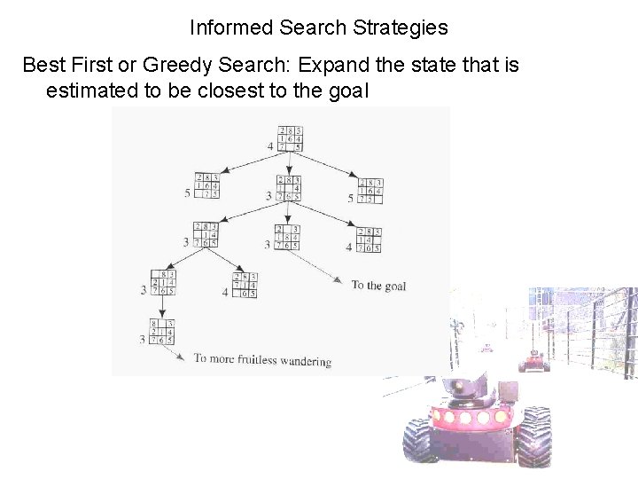
Informed Search Strategies Best First or Greedy Search: Expand the state that is estimated to be closest to the goal

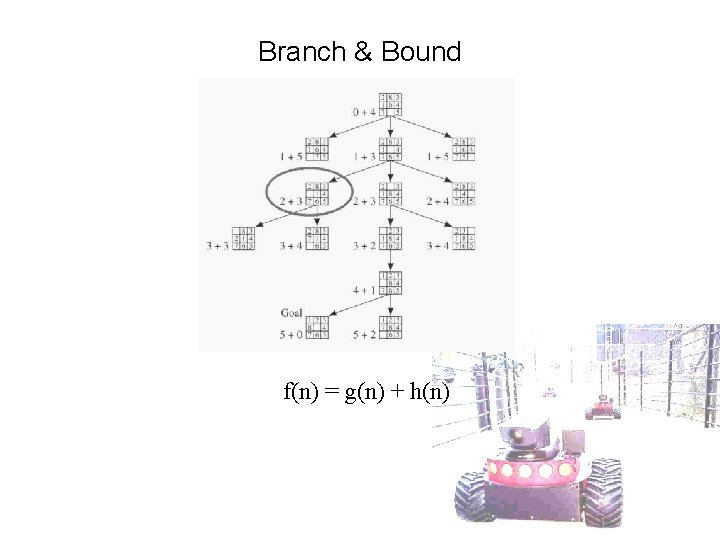
Informed Search Strategies Branch & Bound: Expand the state that is estimated to be closest to the goal f(n) = g(n) + h(n) g(n) = actual cost of path going through state n f(n) is estimated cost of the cheapest solution that goes through state n

Branch & Bound f(n) = g(n) + h(n)

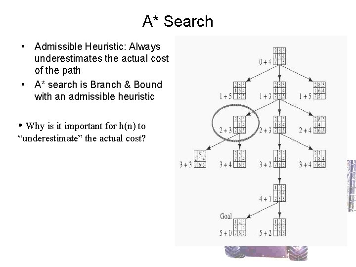
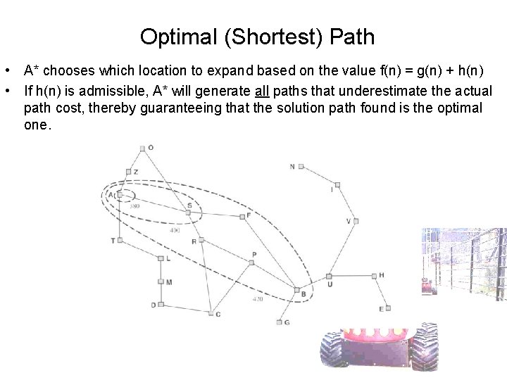
A* Search • Admissible Heuristic: Always underestimates the actual cost of the path • A* search is Branch & Bound with an admissible heuristic • Why is it important for h(n) to “underestimate” the actual cost?

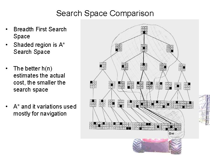
Search Space Comparison • Breadth First Search Space • Shaded region is A* Search Space • The better h(n) estimates the actual cost, the smaller the search space • A* and it variations used mostly for navigation

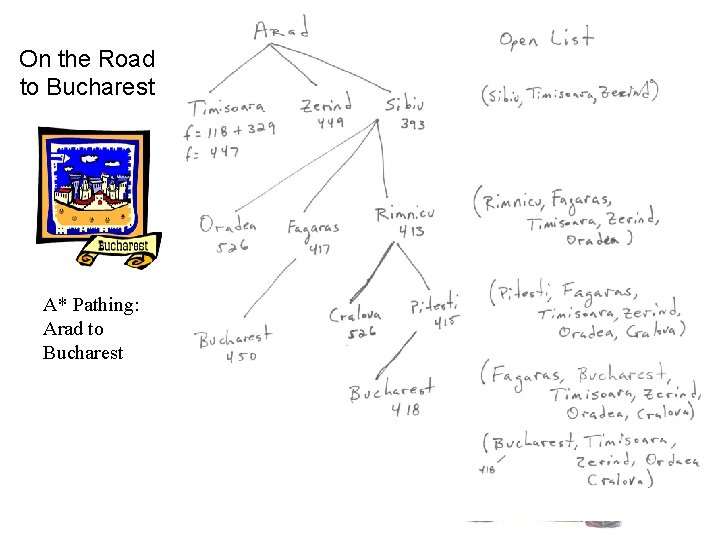
Search: A* • f(n) = g(n) + h(n) – g(n) Cost of going from the starting state to state n – h(n) heuristic estimate of the cost of going from state n to the goal state • Guaranteed to find a solution if one exists • Will find the optimal solution

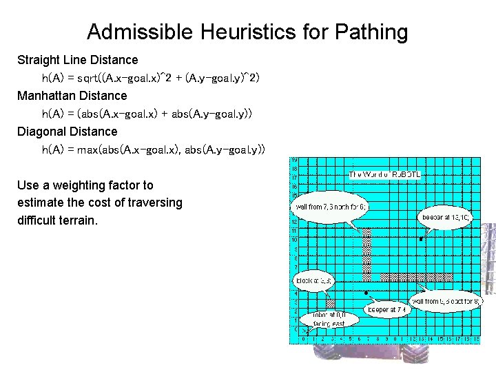
Admissible Heuristics for Pathing Straight Line Distance h(A) = sqrt((A. x-goal. x)^2 + (A. y-goal. y)^2) Manhattan Distance h(A) = (abs(A. x-goal. x) + abs(A. y-goal. y)) Diagonal Distance h(A) = max(abs(A. x-goal. x), abs(A. y-goal. y)) Use a weighting factor to estimate the cost of traversing difficult terrain.

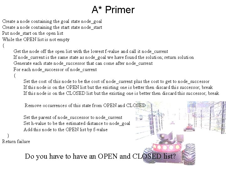
A* Primer Create a node containing the goal state node_goal Create a node containing the start state node_start Put node_start on the open list While the OPEN list is not empty { Get the node off the open list with the lowest f-value and call it node_current If node_current is the same state as node_goal we have found the solution; return solution Generate each state node_successor that can come after node_current For each node_successor of node_current { Set the cost of this node to be the cost of node_current plus the cost to get to node_successor If this node is on the OPEN list but the existing one is better then discard this successor; break If this node is on the CLOSED list but the existing one is better then discard this successor; break Remove occurrences of this state from OPEN and CLOSED Set the parent of node_successor to node_current Set h-value to be the estimated distance to node_goal Add this node to the OPEN list by f-value } Return failure Do you have to have an OPEN and CLOSED list?

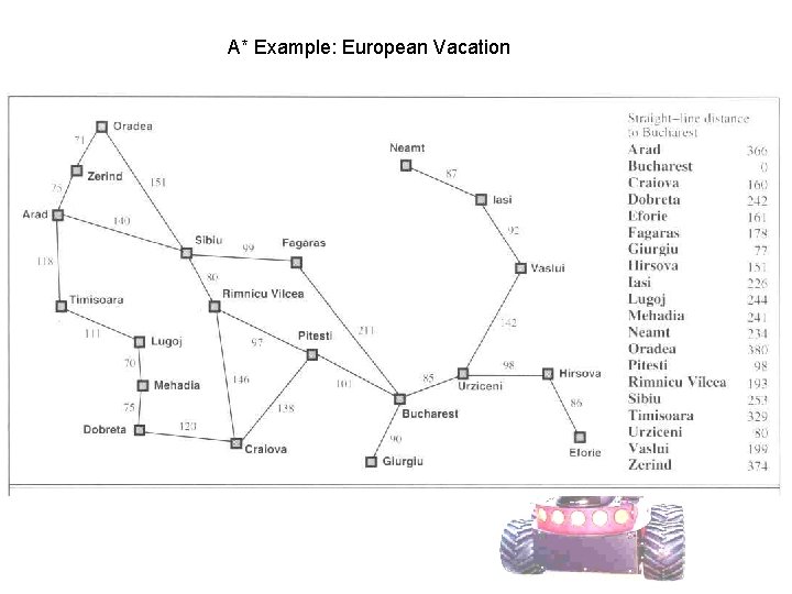
A* Example: European Vacation

On the Road to Bucharest A* Pathing: Arad to Bucharest

Optimal (Shortest) Path • A* chooses which location to expand based on the value f(n) = g(n) + h(n) • If h(n) is admissible, A* will generate all paths that underestimate the actual path cost, thereby guaranteeing that the solution path found is the optimal one.

Additional Points • Cost of Travel – Additional costs associated with path or region. – Terrain – Uphill & down hill costs • An efficient data structure is important for storing the Open and Close lists. – Suggestions? • Variations A* Demo – IDA* (Iterative Deepening) – Bi-directional – D* (Dynamic Planning) – Hierarchical A*

Obstacles • What should the robot do if it cannot complete the plan? • Alternatives – D* – Dijkstra’s Shortest Path Algorithm