Local Search part 2 Haim Kaplan and Uri

Local Search (part 2) Haim Kaplan and Uri Zwick Algorithms in Action Tel Aviv University Last updated: March 31 2016 1

The general scheme • Need to define a neighborhood relation on solutions • Need to find a starting solution • Need to define which neighbor we choose if we have several “improving” ones • Then we “walk’’ from the starting solution to a local optimum 2

Neighborhood size • The neighborhood relation induces a tradeoffs between time and quality • More neighbors ⇒ less local optima but more time per step 3

Back to max-cut • 4

Restarts • If the procedure is fast we can run it from many different starting solutions and pick the best solution found • Starting solutions can be random or perturbations of previous local optima 5

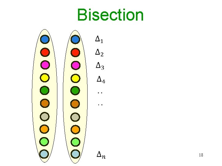
Example: Min-Bisection • 6

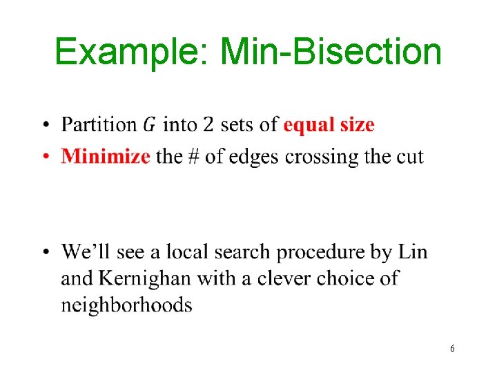
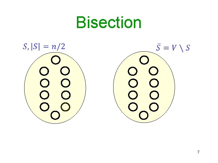
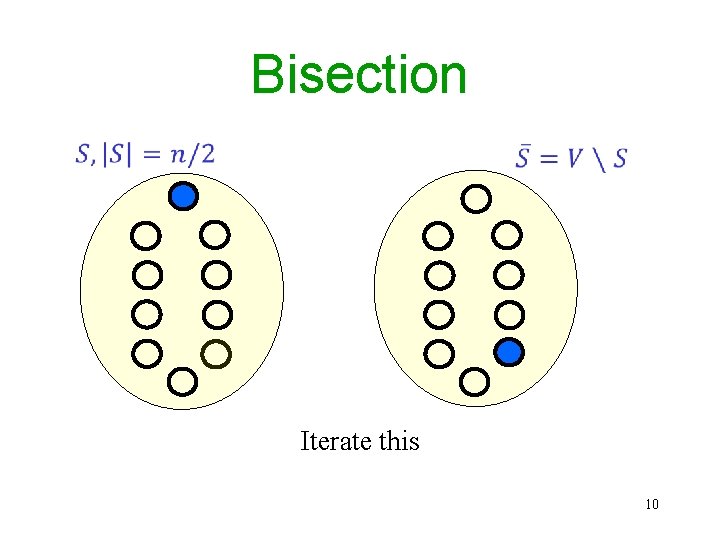
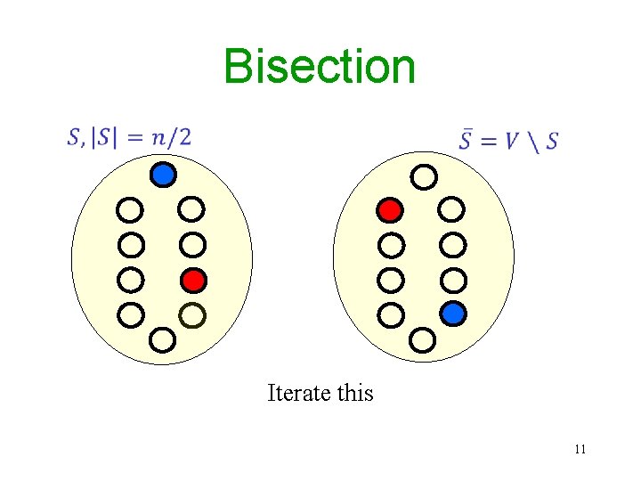
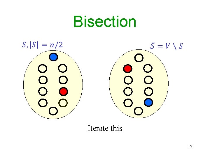
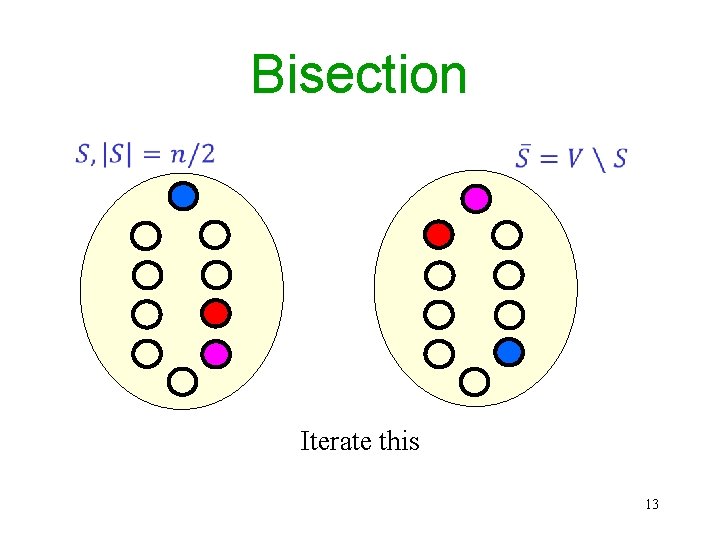
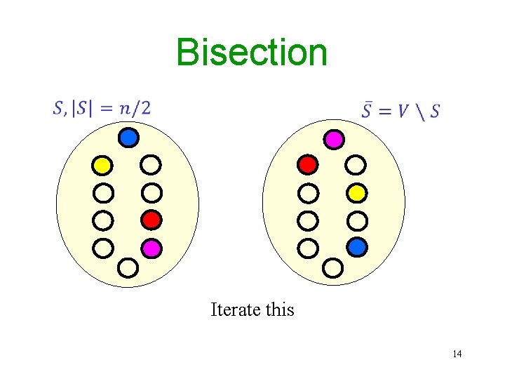
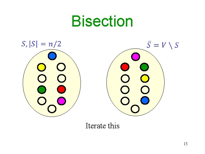
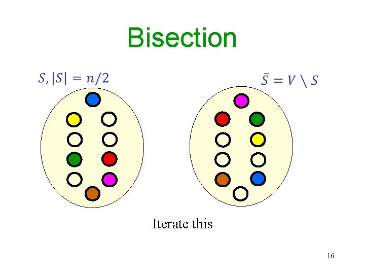
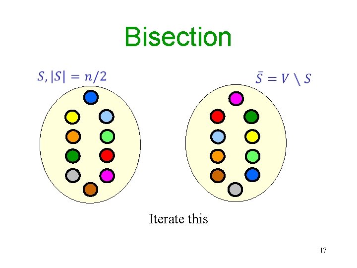
Bisection 7

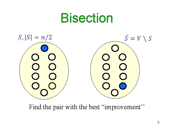
Bisection Find the pair with the best “improvement’’ 8

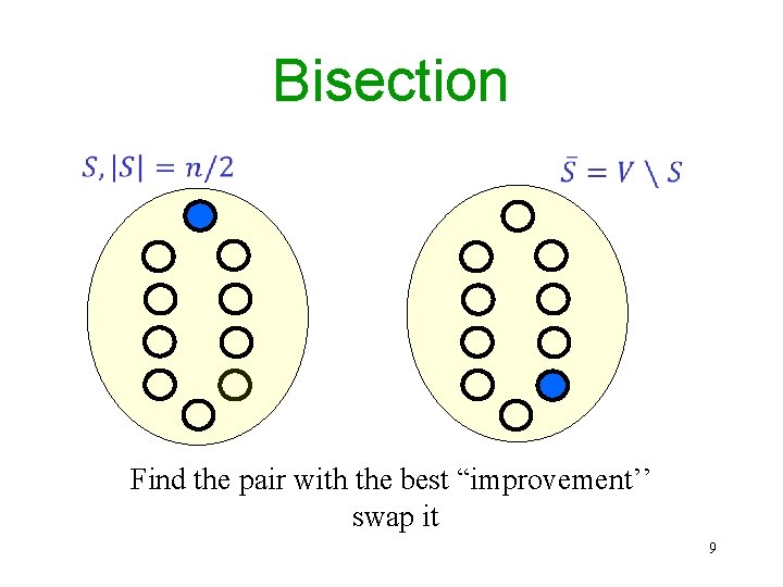
Bisection Find the pair with the best “improvement’’ swap it 9

Bisection Iterate this 10

Bisection Iterate this 11

Bisection Iterate this 12

Bisection Iterate this 13

Bisection Iterate this 14

Bisection Iterate this 15

Bisection Iterate this 16

Bisection Iterate this 17

Bisection 18

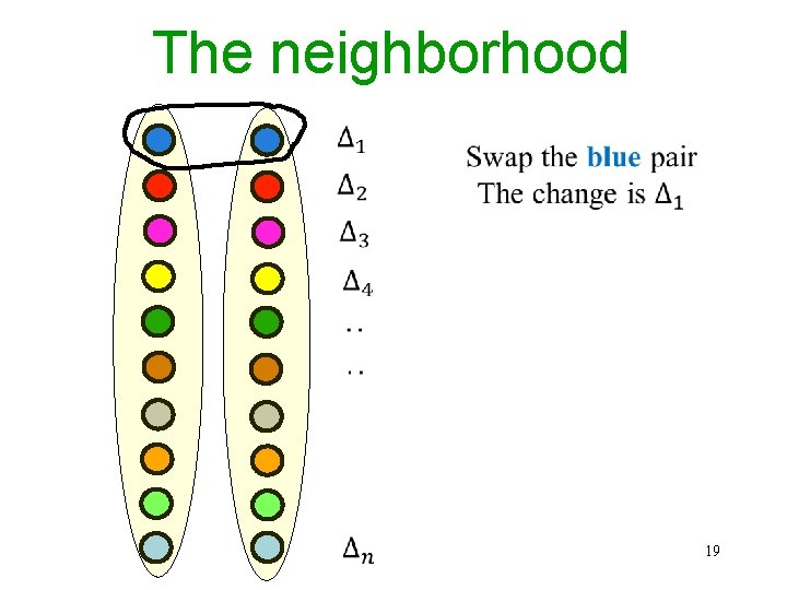
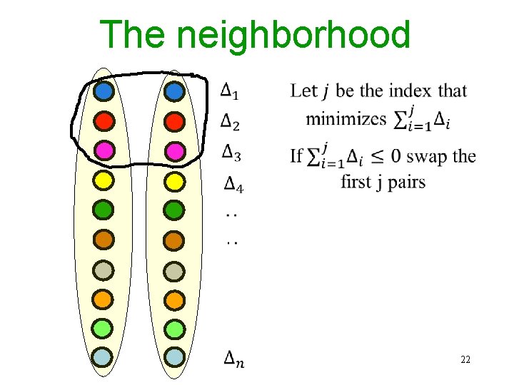
The neighborhood 19

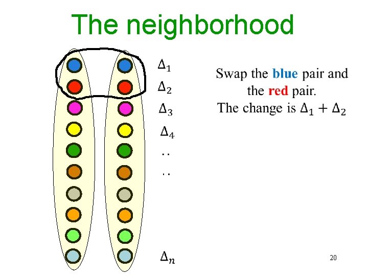
The neighborhood 20

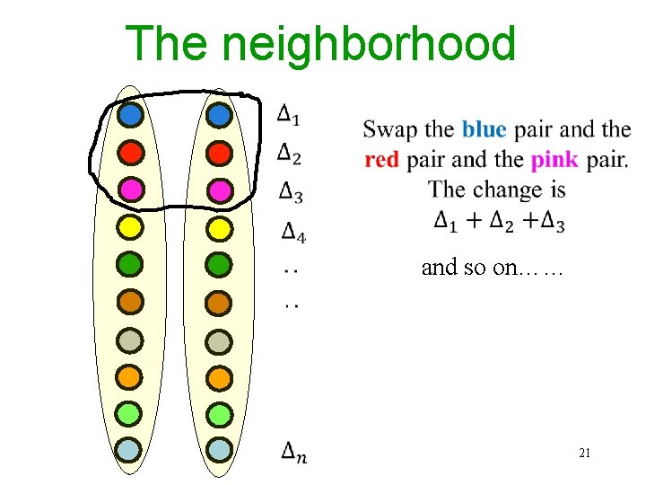
The neighborhood and so on…… 21

The neighborhood 22

Kerninghan-Lin • Unfortunately, a little is known about it theoretically, but • Its quite effective in experiments 23

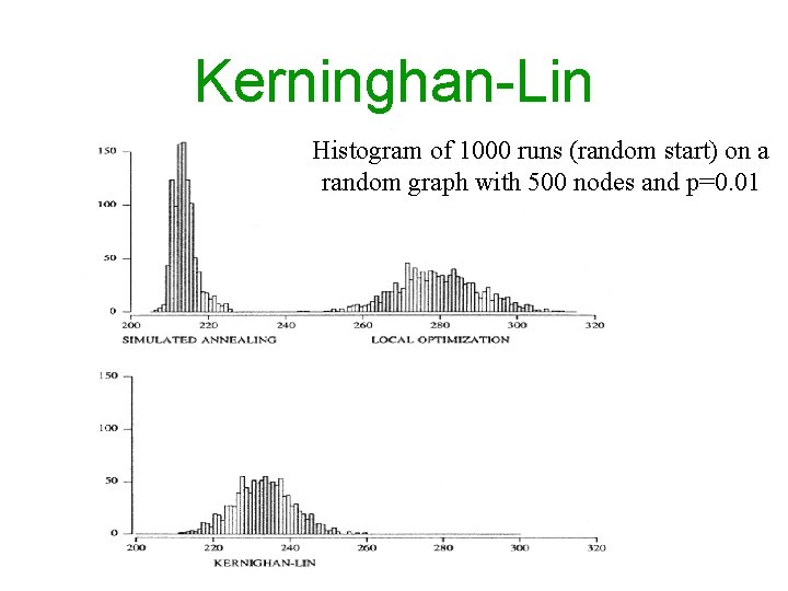
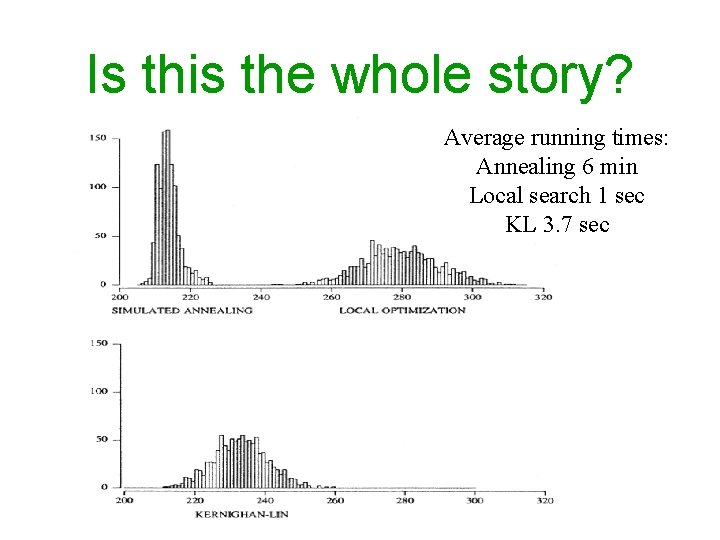
Kerninghan-Lin Histogram of 1000 runs (random start) on a random graph with 500 nodes and p=0. 01

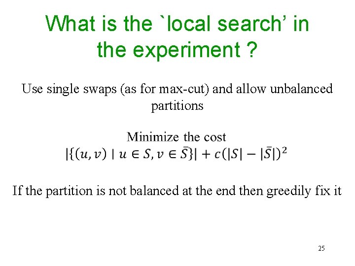
What is the `local search’ in the experiment ? Use single swaps (as for max-cut) and allow unbalanced partitions If the partition is not balanced at the end then greedily fix it 25

Is this the whole story? Average running times: Annealing 6 min Local search 1 sec KL 3. 7 sec

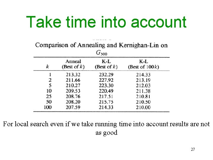
Take time into account For local search even if we take running time into account results are not as good 27

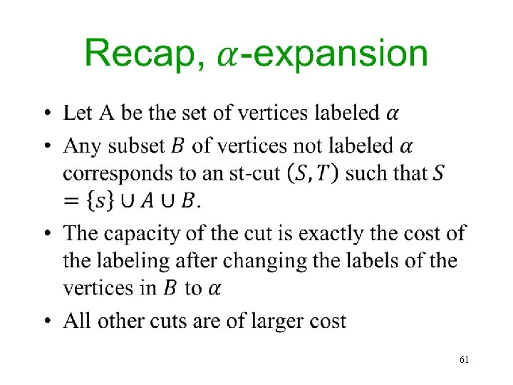
Examples that you have seen. . • 28

Applications in graphics • Image segmentation (2 D, 3 D) • Stereo – depth estimation • There are many others…

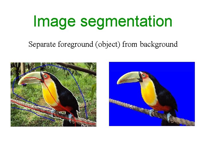
Image segmentation Separate foreground (object) from background

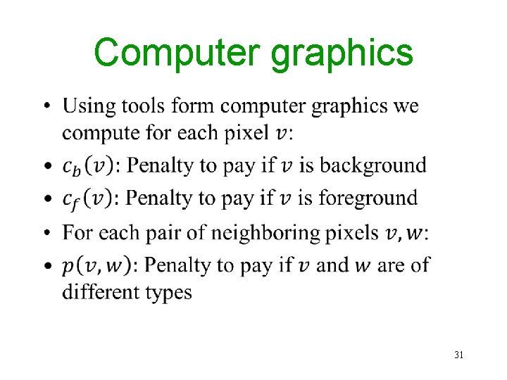
Computer graphics • 31

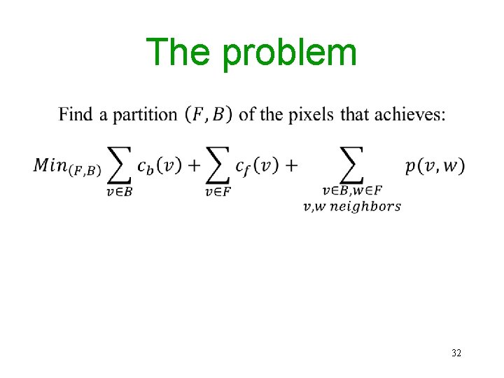
The problem 32

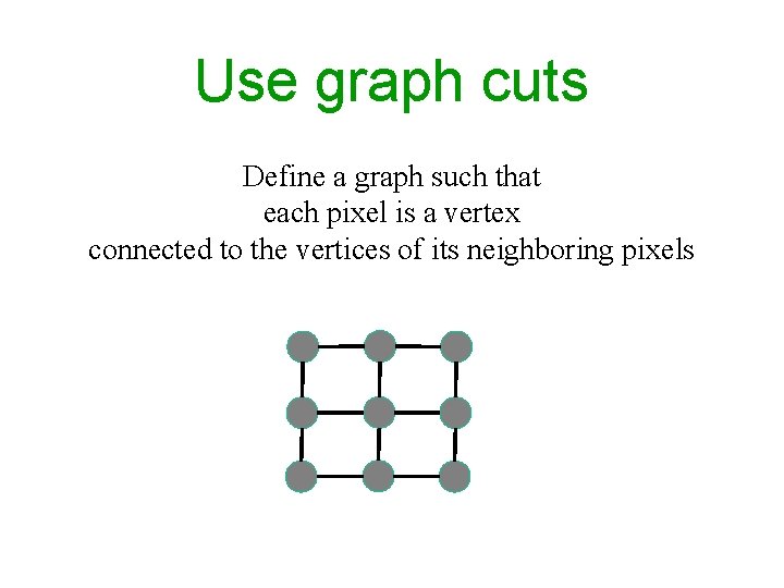
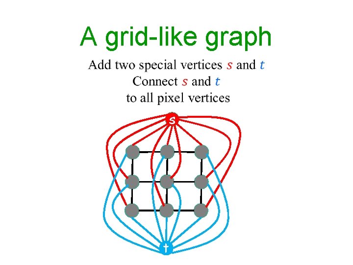
Use graph cuts Define a graph such that each pixel is a vertex connected to the vertices of its neighboring pixels

A grid-like graph s t

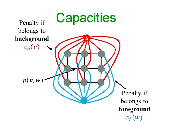
Capacities s t

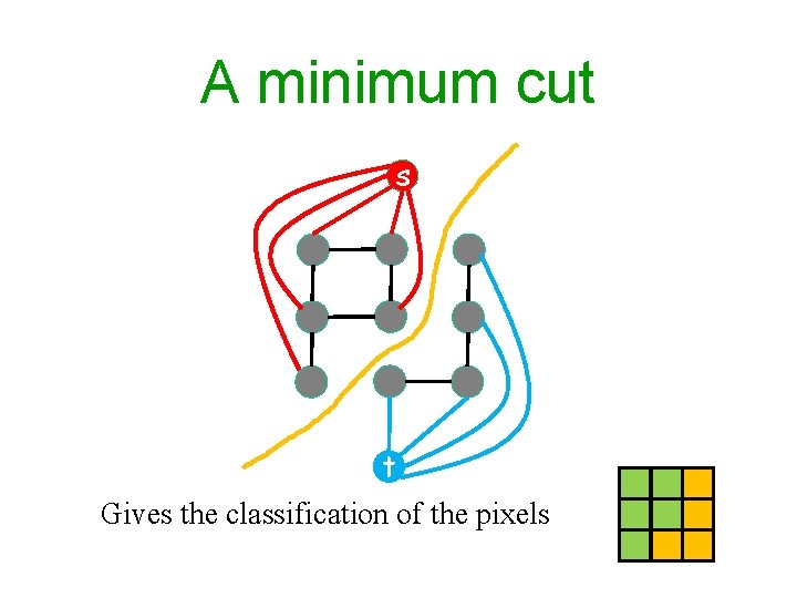
A minimum cut s t Gives the classification of the pixels

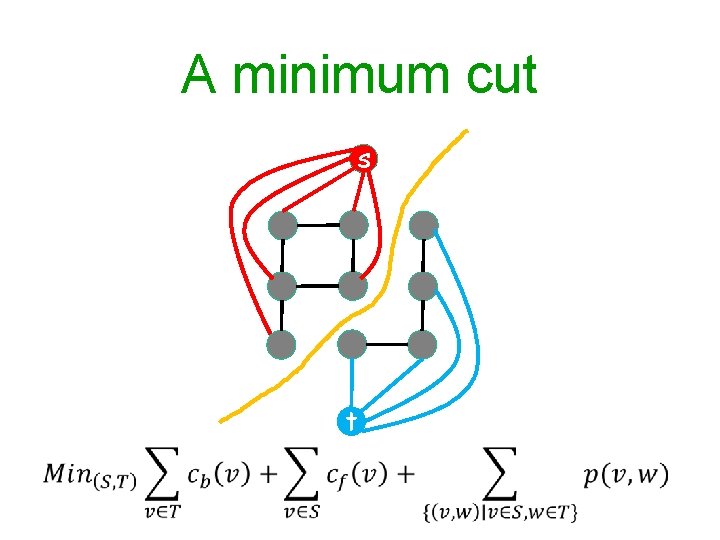
A minimum cut s t

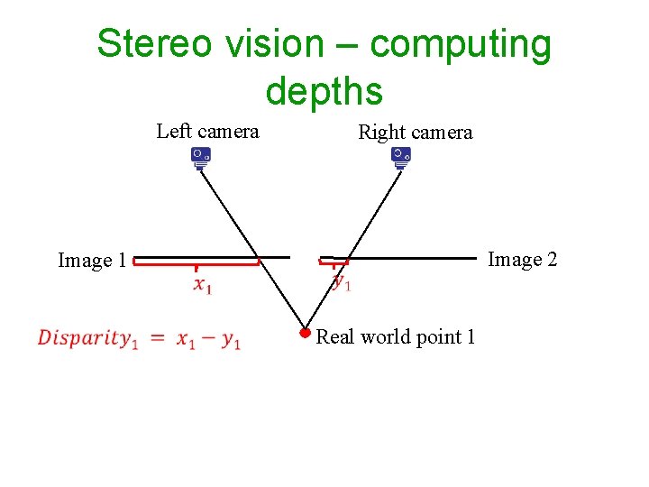
Stereo vision – computing depths Left camera Image 1 Right camera Real world point 1 Image 2

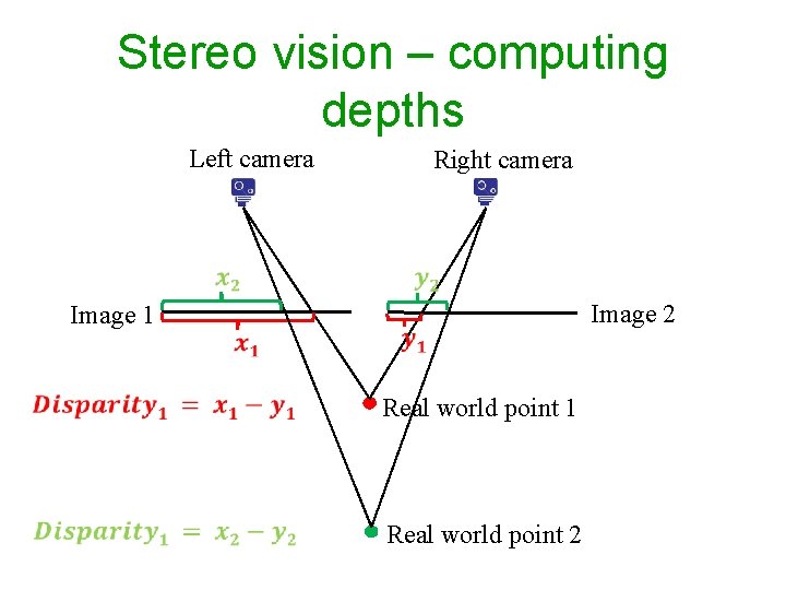
Stereo vision – computing depths Left camera Right camera Image 1 Real world point 1 Real world point 2 Image 2

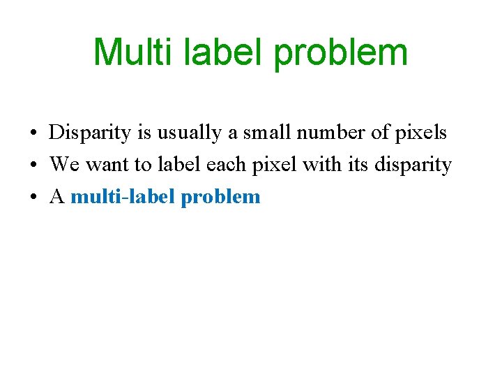
Multi label problem • Disparity is usually a small number of pixels • We want to label each pixel with its disparity • A multi-label problem

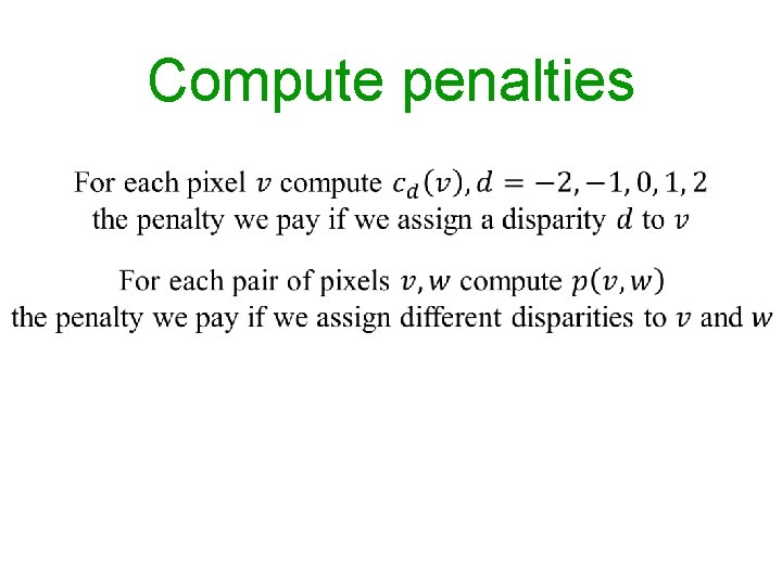
Compute penalties

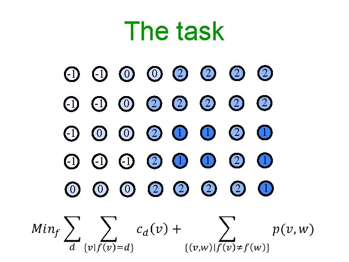
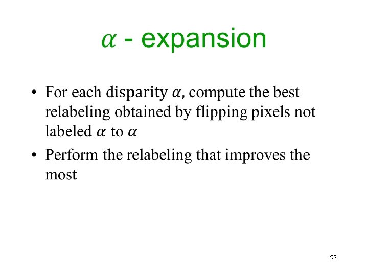
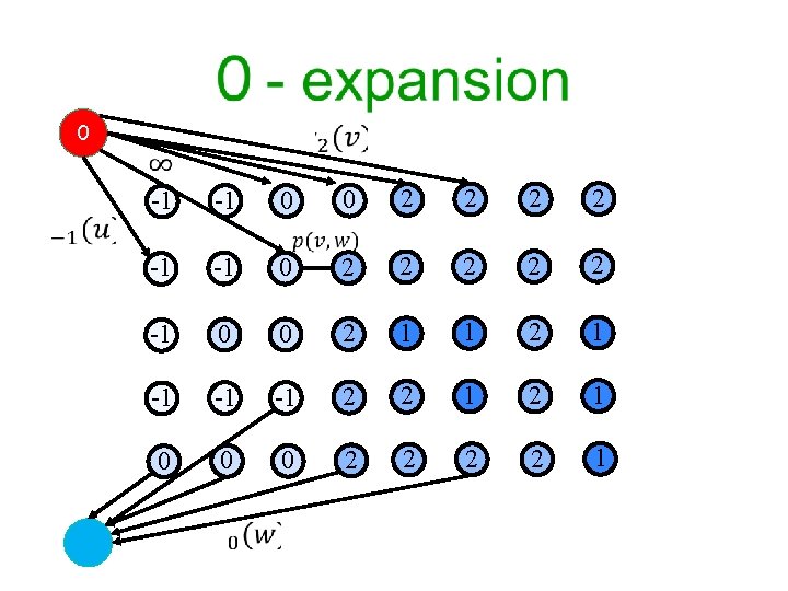
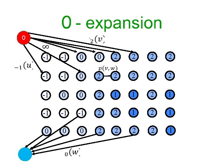
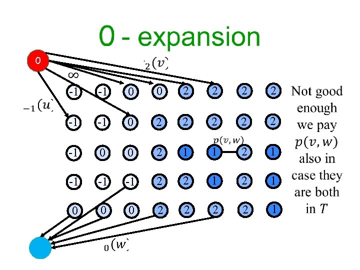
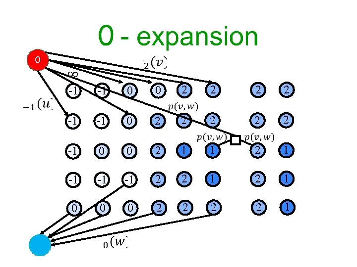
The task -1 -1 0 0 2 2 -1 -1 0 2 2 2 -1 0 0 2 1 1 2 1 -1 -1 -1 2 1 0 0 0 2 2 1

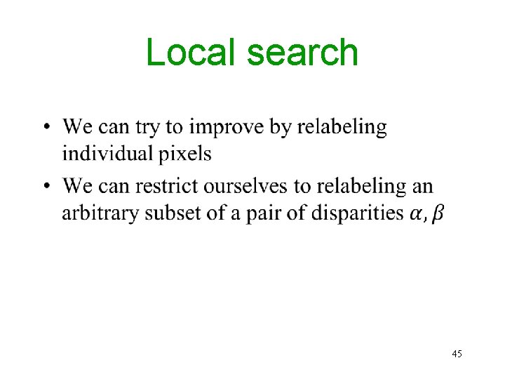
Local search • 45

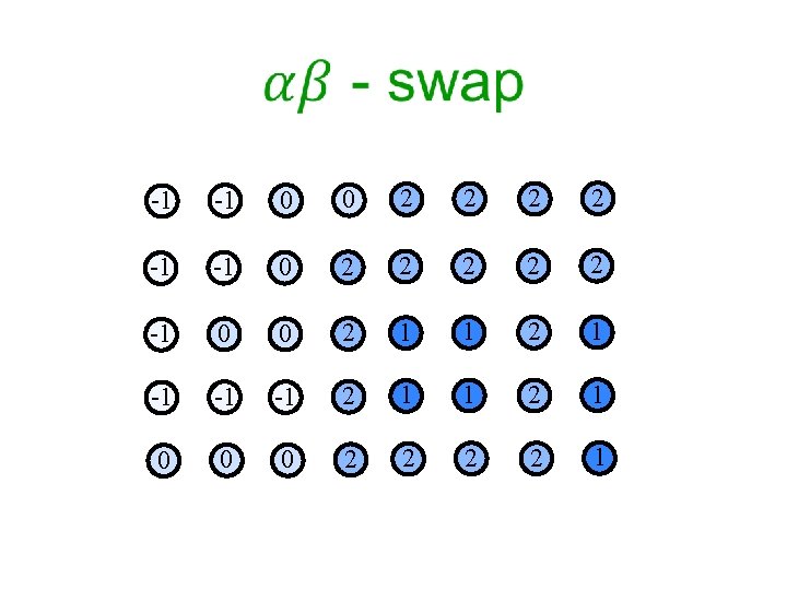
-1 -1 0 0 2 2 -1 -1 0 2 2 2 -1 0 0 2 1 1 2 1 -1 -1 -1 2 1 0 0 0 2 2 1

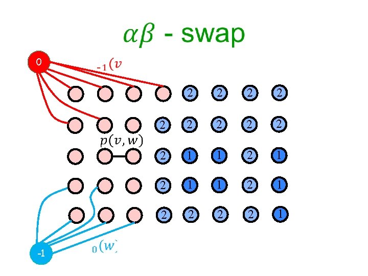
0 2 2 2 2 2 1 1 2 1 2 2 2 2 1 -1

Theory ? 49

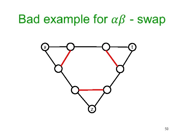
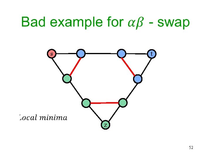
s t z 50

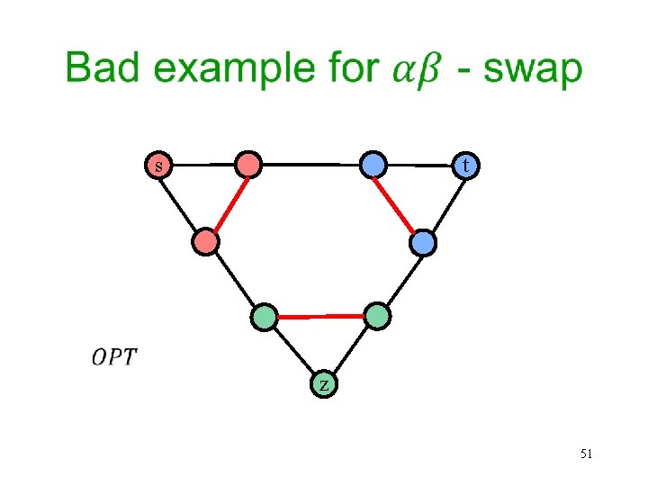
s t z 51

s t z 52

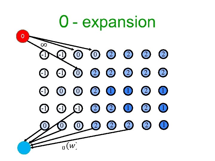
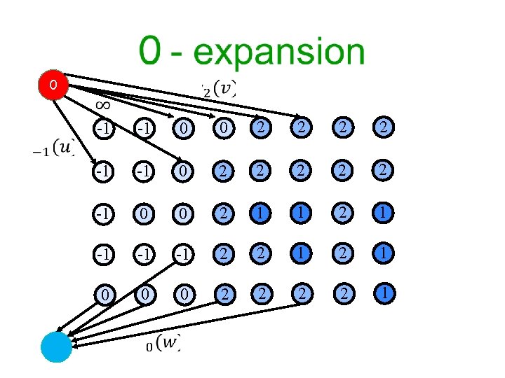
0 -1 -1 0 0 2 2 -1 -1 0 2 2 2 -1 0 0 2 1 1 2 1 -1 -1 -1 2 2 1 0 0 0 2 2 1

0 -1 -1 0 0 2 2 -1 -1 0 2 2 2 -1 0 0 2 1 1 2 1 -1 -1 -1 2 2 1 0 0 0 2 2 1

0 -1 -1 0 0 2 2 -1 -1 0 2 2 2 -1 0 0 2 1 1 2 1 -1 -1 -1 2 2 1 0 0 0 2 2 1

0 -1 -1 0 0 2 2 -1 -1 0 2 2 2 -1 0 0 2 1 1 2 1 -1 -1 -1 2 2 1 0 0 0 2 2 1

0 -1 -1 0 0 2 2 -1 -1 0 2 2 2 -1 0 0 2 1 1 2 1 -1 -1 -1 2 2 1 0 0 0 2 2 1

0 -1 -1 -1 0 0 2 2 2 2 2 1 1 -1 0 0 2 1 -1 -1 -1 2 2 1 0 0 0 2 2 1

Theory ? 62

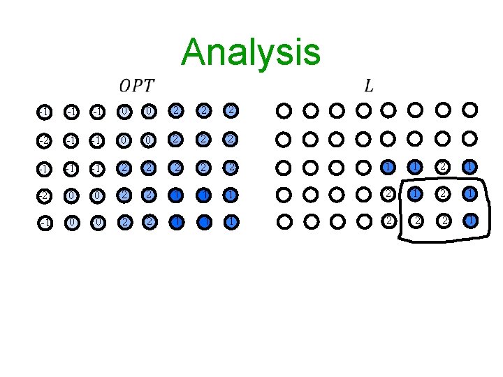
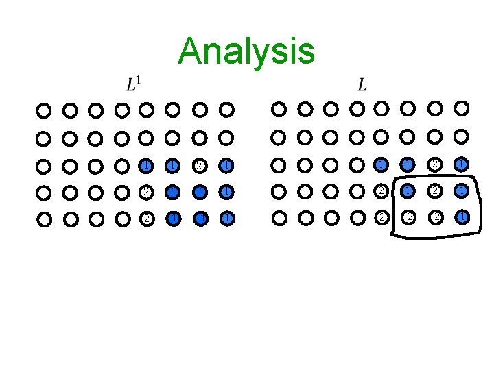
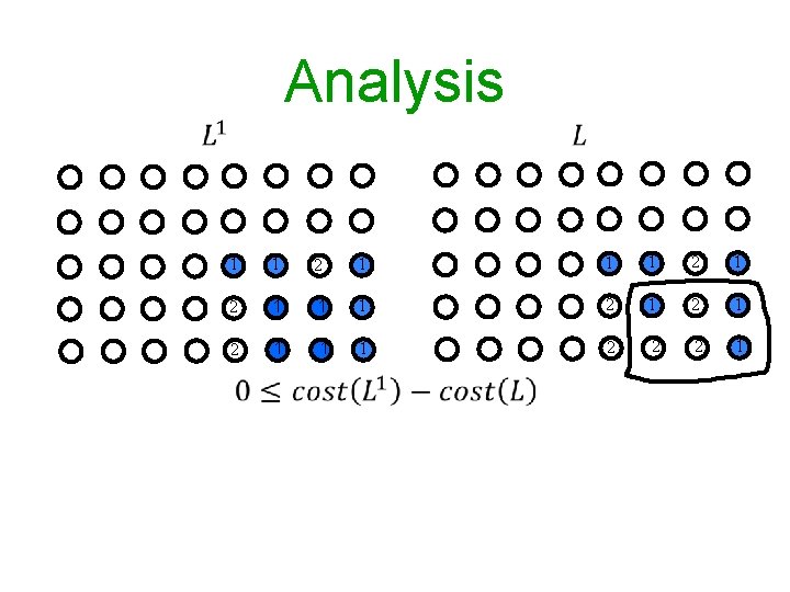
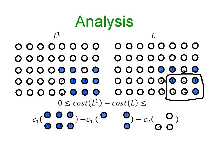
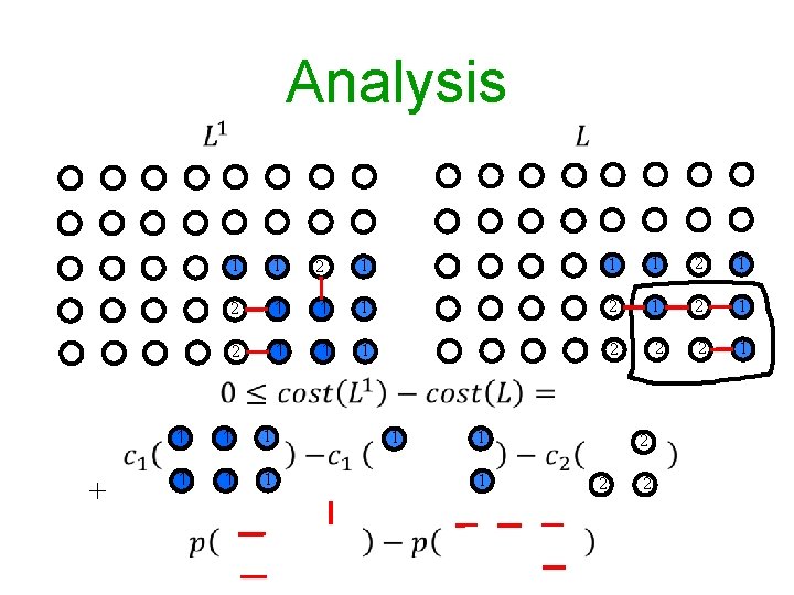
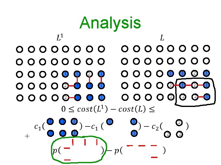
Analysis 2 1 1 2 1 1 1 2 2 2 1 -1 -1 -1 0 0 2 2 2 -2 -1 -1 0 0 2 2 2 -1 -1 -1 2 2 -2 0 0 2 2 1 -1 0 0 2 2 1

Analysis 1 1 1 2 1 1 1 2 2 2 1 1 1 2 2 1

Analysis 1 1 1 2 1 1 1 2 2 2 1 1 1 2 2 1

Analysis 1 1 1 2 1 1 1 2 2 2 1 1 1 2 2 1 1 1 1 1 1 1 2 2 2

Analysis 1 1 1 2 1 1 1 2 2 2 1 1 1 2 2 1 + 1 1 1 1 1 1 2 2 2

Analysis 1 1 1 2 1 1 1 2 2 2 1 1 1 2 2 1 + 1 1 1 1 1 1 2 2 2

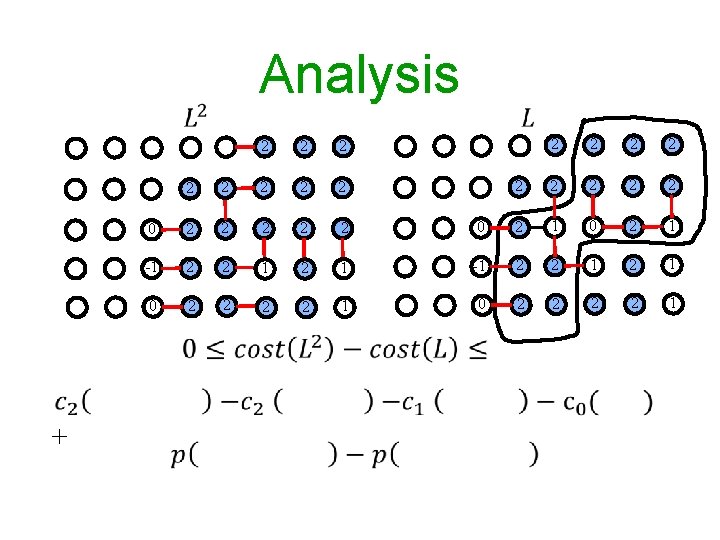
Analysis 2 2 2 2 2 0 2 1 -1 2 2 1 0 2 2 1 2 2 2 2 2 0 2 2 2 -1 2 2 1 0 2 2 1 +

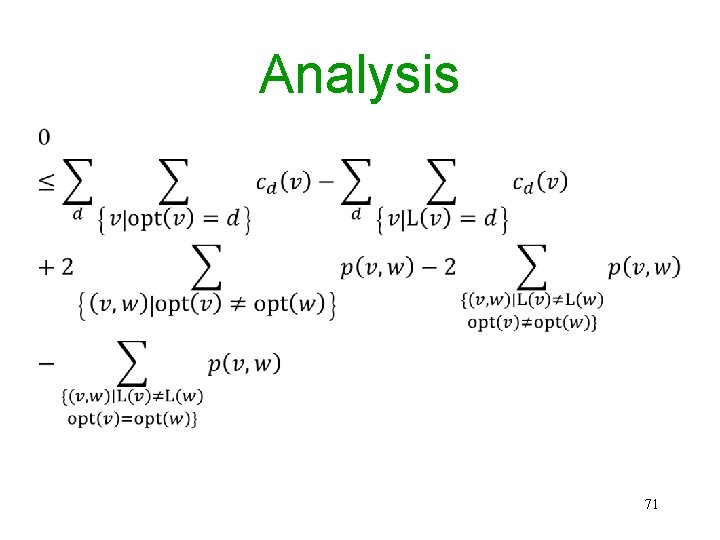
Analysis 71

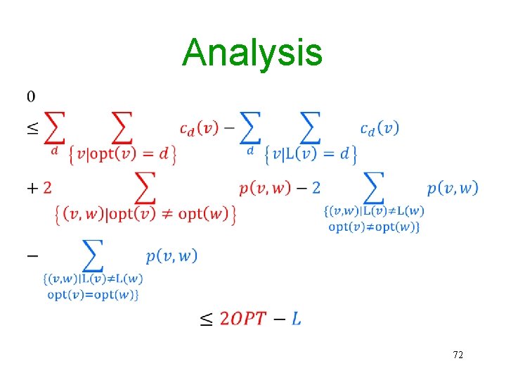
Analysis 72