Local features main components 1 Detection Find a

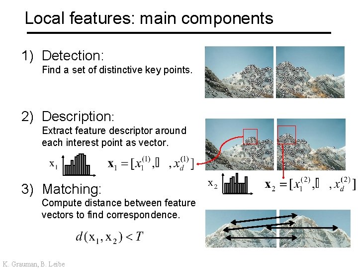
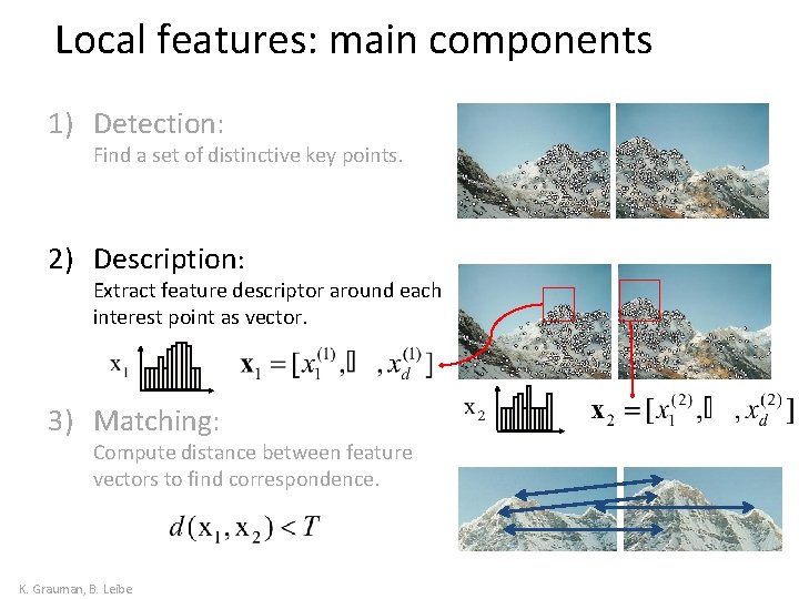
Local features: main components 1) Detection: Find a set of distinctive key points. 2) Description: Extract feature descriptor around each interest point as vector. 3) Matching: Compute distance between feature vectors to find correspondence. K. Grauman, B. Leibe

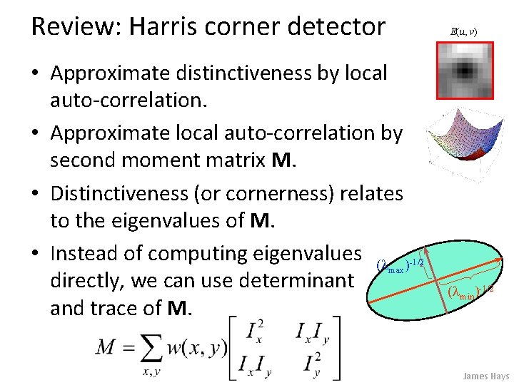
Review: Harris corner detector • Approximate distinctiveness by local auto-correlation. • Approximate local auto-correlation by second moment matrix M. • Distinctiveness (or cornerness) relates to the eigenvalues of M. • Instead of computing eigenvalues ( )-1/2 max directly, we can use determinant and trace of M. E(u, v) ( min)-1/2 James Hays

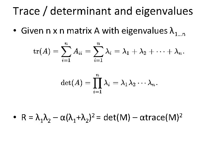
Trace / determinant and eigenvalues • Given n x n matrix A with eigenvalues λ 1…n • R = λ 1λ 2 – α(λ 1+λ 2)2 = det(M) – αtrace(M)2

Harris Detector [Harris 88] 1. Image derivatives (optionally, blur first) Ix Iy Ix 2 Iy 2 Ix Iy g(Ix 2) g(Iy 2) g(Ix. Iy) 2. Square of derivatives 3. Gaussian filter g(s. I) 4. Cornerness function – both eigenvalues are strong 5. Non-maxima suppression 5 har James Hays

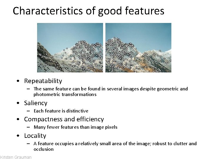
Characteristics of good features • Repeatability – The same feature can be found in several images despite geometric and photometric transformations • Saliency – Each feature is distinctive • Compactness and efficiency – Many fewer features than image pixels • Locality – A feature occupies a relatively small area of the image; robust to clutter and occlusion Kristen Grauman

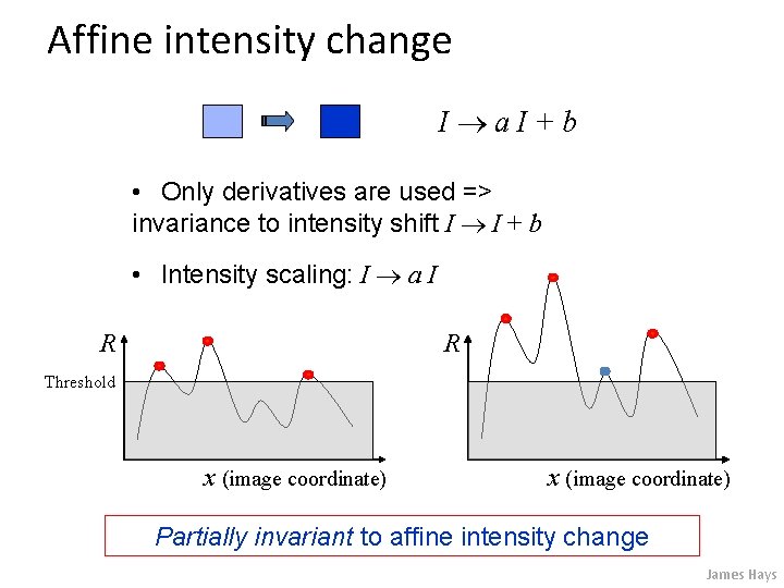
Affine intensity change I a. I+b • Only derivatives are used => invariance to intensity shift I I + b • Intensity scaling: I a I R R Threshold x (image coordinate) Partially invariant to affine intensity change James Hays

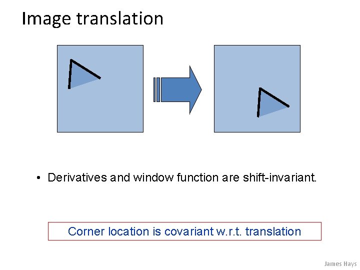
Image translation • Derivatives and window function are shift-invariant. Corner location is covariant w. r. t. translation James Hays

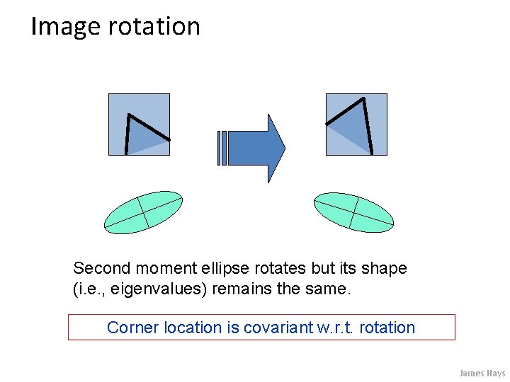
Image rotation Second moment ellipse rotates but its shape (i. e. , eigenvalues) remains the same. Corner location is covariant w. r. t. rotation James Hays

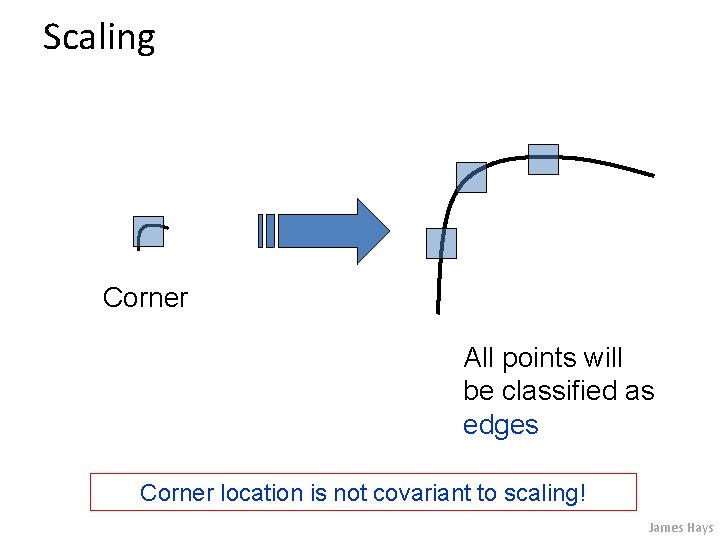
Scaling Corner All points will be classified as edges Corner location is not covariant to scaling! James Hays

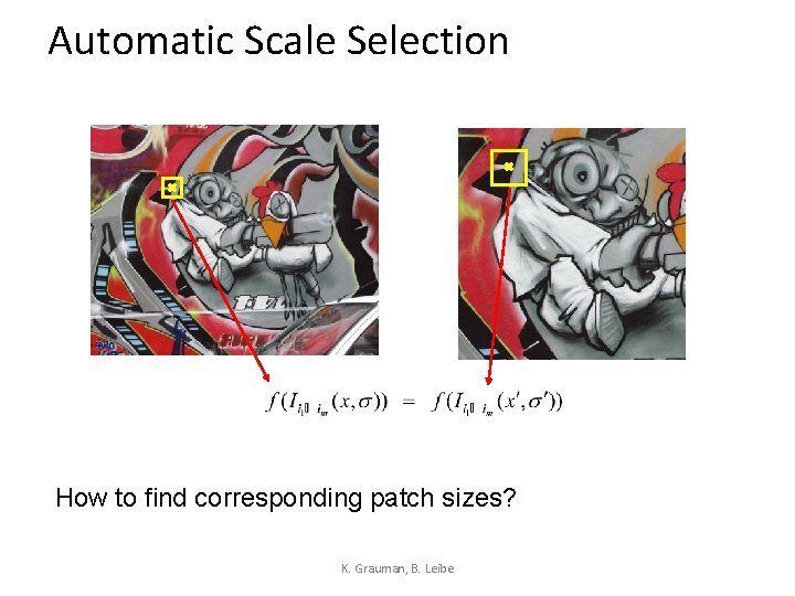
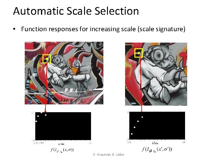
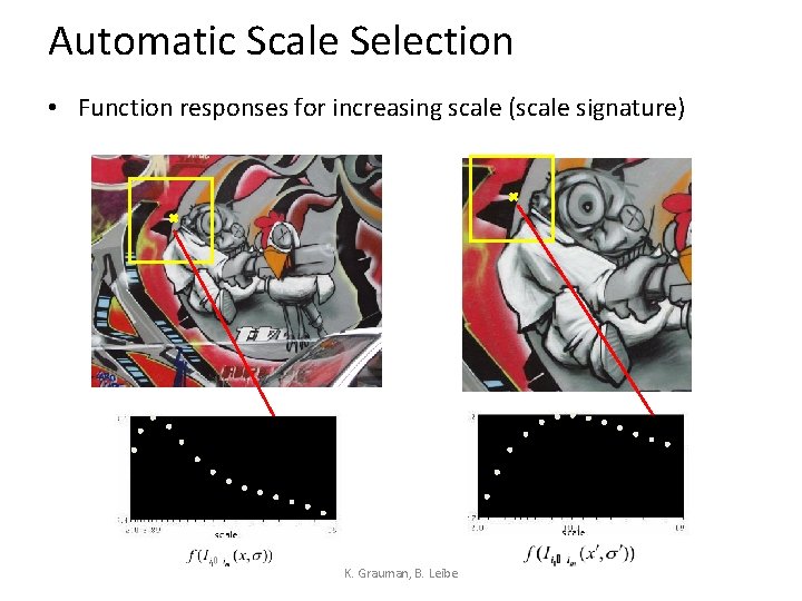
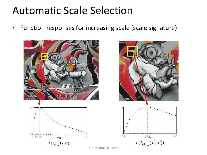
Automatic Scale Selection How to find corresponding patch sizes? K. Grauman, B. Leibe

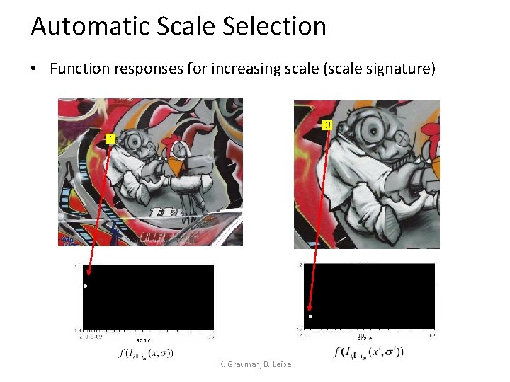
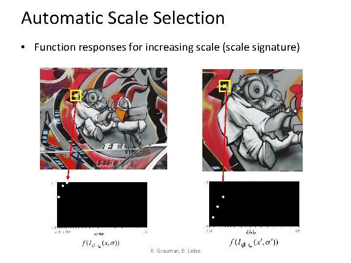
Automatic Scale Selection • Function responses for increasing scale (scale signature) K. Grauman, B. Leibe

Automatic Scale Selection • Function responses for increasing scale (scale signature) K. Grauman, B. Leibe

Automatic Scale Selection • Function responses for increasing scale (scale signature) K. Grauman, B. Leibe

Automatic Scale Selection • Function responses for increasing scale (scale signature) K. Grauman, B. Leibe

Automatic Scale Selection • Function responses for increasing scale (scale signature) K. Grauman, B. Leibe

Automatic Scale Selection • Function responses for increasing scale (scale signature) K. Grauman, B. Leibe

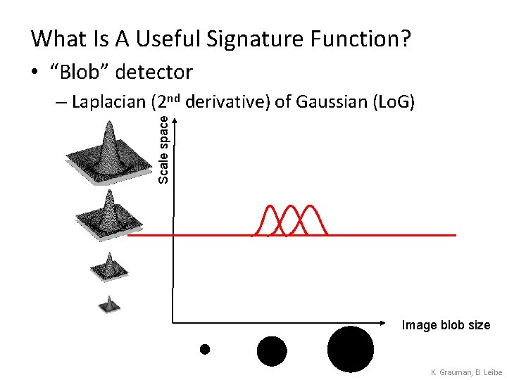
What Is A Useful Signature Function? • “Blob” detector Scale space – Laplacian (2 nd derivative) of Gaussian (Lo. G) Image blob size K. Grauman, B. Leibe

Find local maxima in position-scale space s 5 Find maxima s 4 s 3 s 2 List of (x, y, s) s K. Grauman, B. Leibe

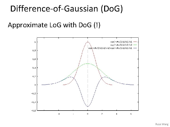
Difference-of-Gaussian (Do. G) Approximate Lo. G with Do. G (!) Ruye Wang

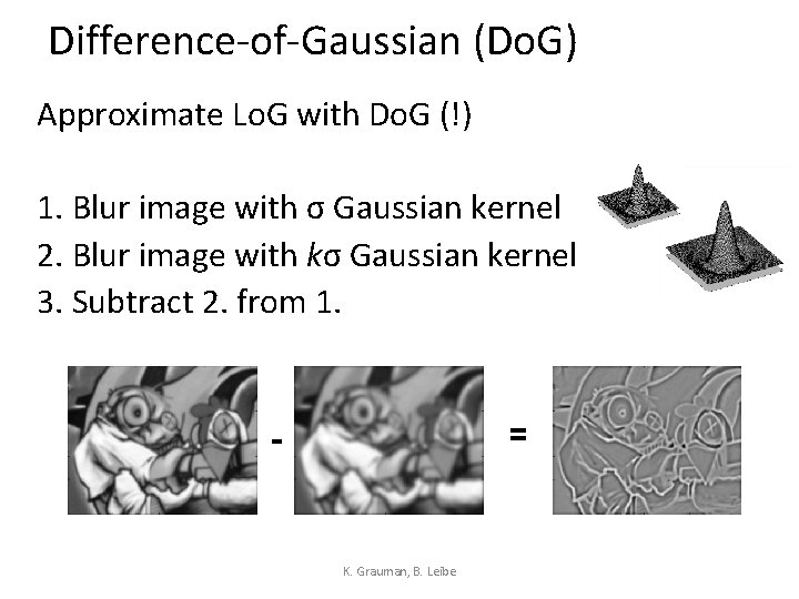
Difference-of-Gaussian (Do. G) Approximate Lo. G with Do. G (!) 1. Blur image with σ Gaussian kernel 2. Blur image with kσ Gaussian kernel 3. Subtract 2. from 1. = - K. Grauman, B. Leibe

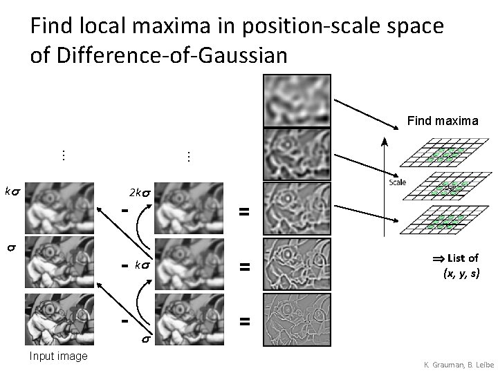
Find local maxima in position-scale space of Difference-of-Gaussian ks … … Find maxima - s Input image 2 ks = ks s = List of (x, y, s) = K. Grauman, B. Leibe

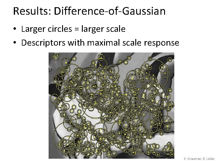
Results: Difference-of-Gaussian • Larger circles = larger scale • Descriptors with maximal scale response K. Grauman, B. Leibe

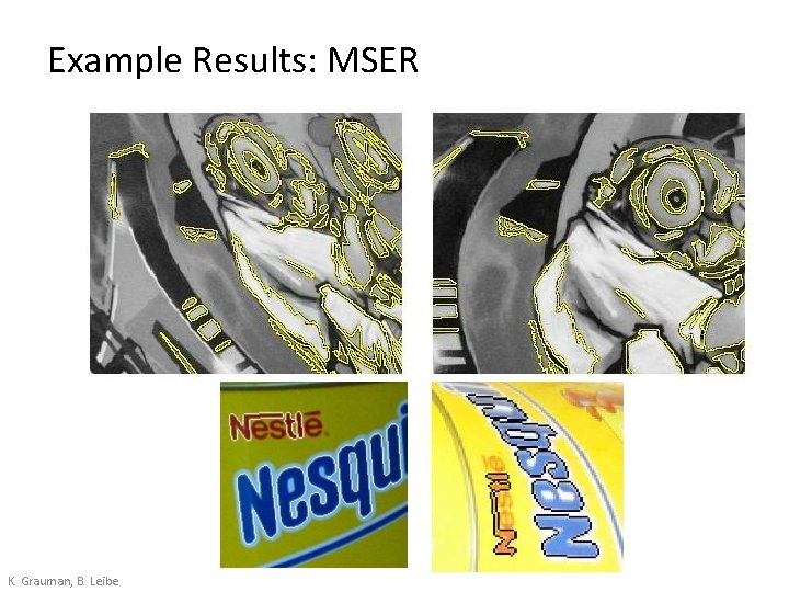
Maximally Stable Extremal Regions [Matas ‘ 02] • Based on Watershed segmentation algorithm • Select regions that stay stable over a large parameter range K. Grauman, B. Leibe

Example Results: MSER K. Grauman, B. Leibe

Local Image Descriptors Read Szeliski 4. 1 Acknowledgment: Many slides from James Hays, Derek Hoiem and Grauman & Leibe 2008 AAAI Tutorial

Local features: main components 1) Detection: Find a set of distinctive key points. 2) Description: Extract feature descriptor around each interest point as vector. 3) Matching: Compute distance between feature vectors to find correspondence. K. Grauman, B. Leibe

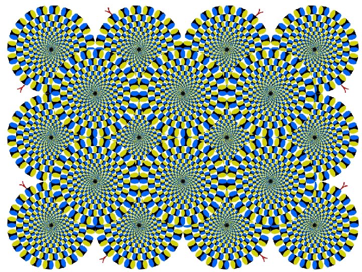
Motion illusion, rotating snakes

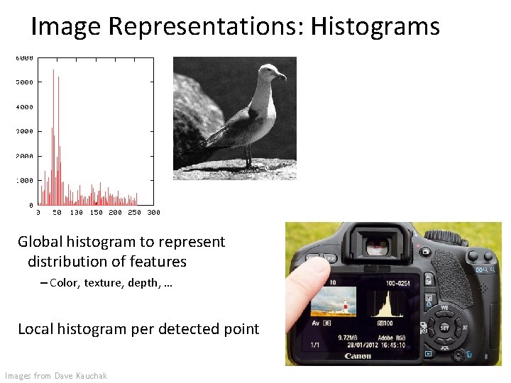
Image Representations: Histograms Global histogram to represent distribution of features – Color, texture, depth, … Local histogram per detected point Images from Dave Kauchak Space Shuttle Cargo Bay

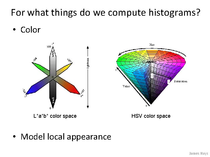
For what things do we compute histograms? • Color L*a*b* color space HSV color space • Model local appearance James Hays

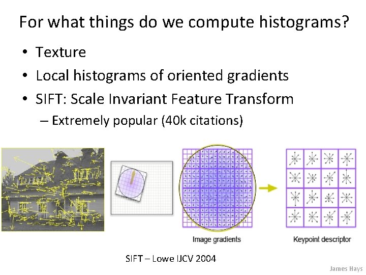
For what things do we compute histograms? • Texture • Local histograms of oriented gradients • SIFT: Scale Invariant Feature Transform – Extremely popular (40 k citations) SIFT – Lowe IJCV 2004 James Hays

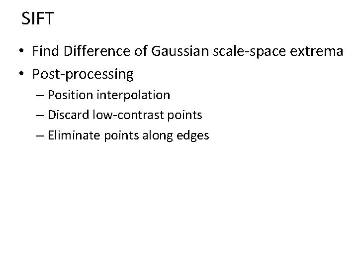
SIFT • Find Difference of Gaussian scale-space extrema • Post-processing – Position interpolation – Discard low-contrast points – Eliminate points along edges

SIFT • Find Difference of Gaussian scale-space extrema • Post-processing – Position interpolation – Discard low-contrast points – Eliminate points along edges • Orientation estimation

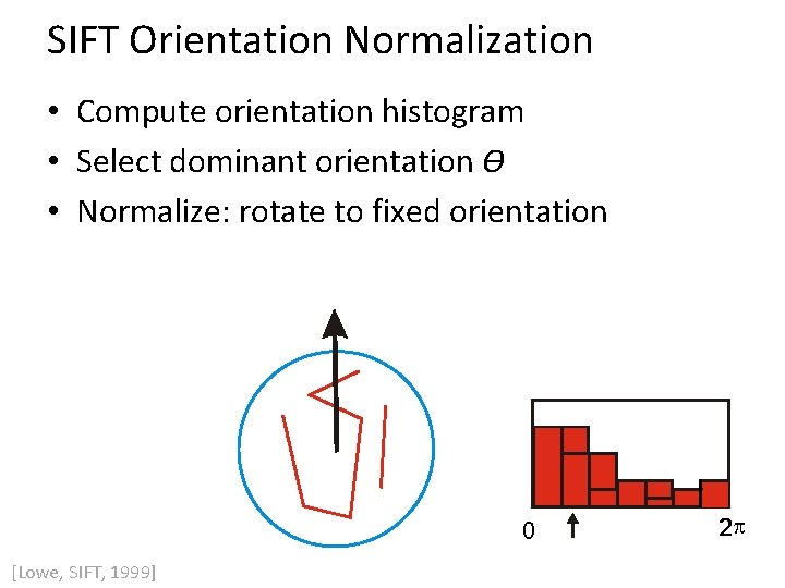
SIFT Orientation Normalization • Compute orientation histogram • Select dominant orientation ϴ • Normalize: rotate to fixed orientation 0 [Lowe, SIFT, 1999] T. Tuytelaars, B. Leibe 2 p

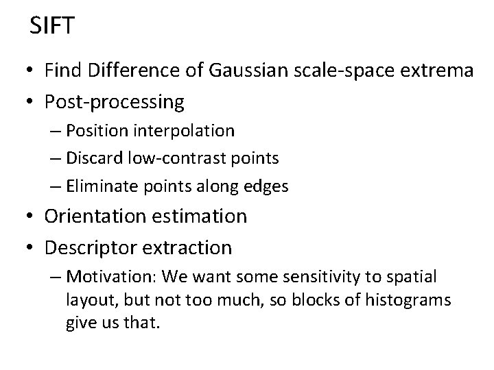
SIFT • Find Difference of Gaussian scale-space extrema • Post-processing – Position interpolation – Discard low-contrast points – Eliminate points along edges • Orientation estimation • Descriptor extraction – Motivation: We want some sensitivity to spatial layout, but not too much, so blocks of histograms give us that.

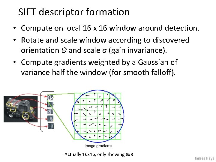
SIFT descriptor formation • Compute on local 16 x 16 window around detection. • Rotate and scale window according to discovered orientation ϴ and scale σ (gain invariance). • Compute gradients weighted by a Gaussian of variance half the window (for smooth falloff). Actually 16 x 16, only showing 8 x 8 James Hays

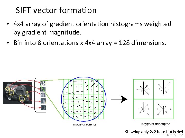
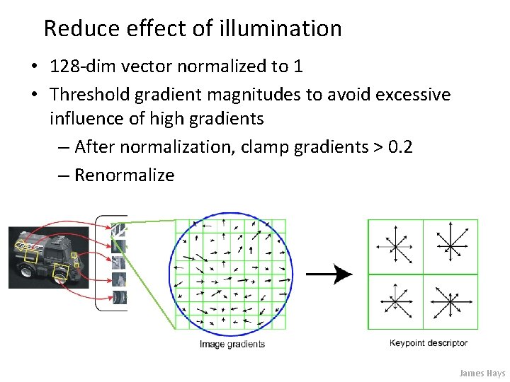
SIFT vector formation • 4 x 4 array of gradient orientation histograms weighted by gradient magnitude. • Bin into 8 orientations x 4 x 4 array = 128 dimensions. Showing only 2 x 2 here but is 4 x 4 James Hays

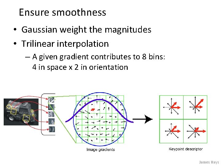
Ensure smoothness • Gaussian weight the magnitudes • Trilinear interpolation – A given gradient contributes to 8 bins: 4 in space x 2 in orientation James Hays

Reduce effect of illumination • 128 -dim vector normalized to 1 • Threshold gradient magnitudes to avoid excessive influence of high gradients – After normalization, clamp gradients > 0. 2 – Renormalize James Hays

SIFT-like descriptor in Project 2 • SIFT is hand designed based on intuition • You implement your own SIFT-like descriptor • May be some trial and error • Feel free to look at papers / resources for inspiration 50

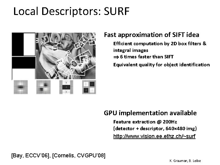
Local Descriptors: SURF • Fast approximation of SIFT idea Ø Ø Efficient computation by 2 D box filters & integral images 6 times faster than SIFT Equivalent quality for object identification • GPU implementation available Ø Ø [Bay, ECCV’ 06], [Cornelis, CVGPU’ 08] Feature extraction @ 200 Hz (detector + descriptor, 640× 480 img) http: //www. vision. ee. ethz. ch/~surf K. Grauman, B. Leibe

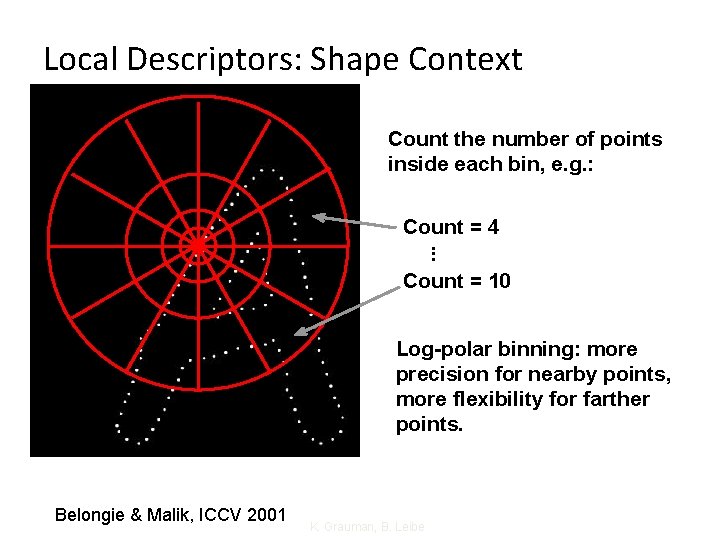
Local Descriptors: Shape Context Count the number of points inside each bin, e. g. : Count = 4. . . Count = 10 Log-polar binning: more precision for nearby points, more flexibility for farther points. Belongie & Malik, ICCV 2001 K. Grauman, B. Leibe

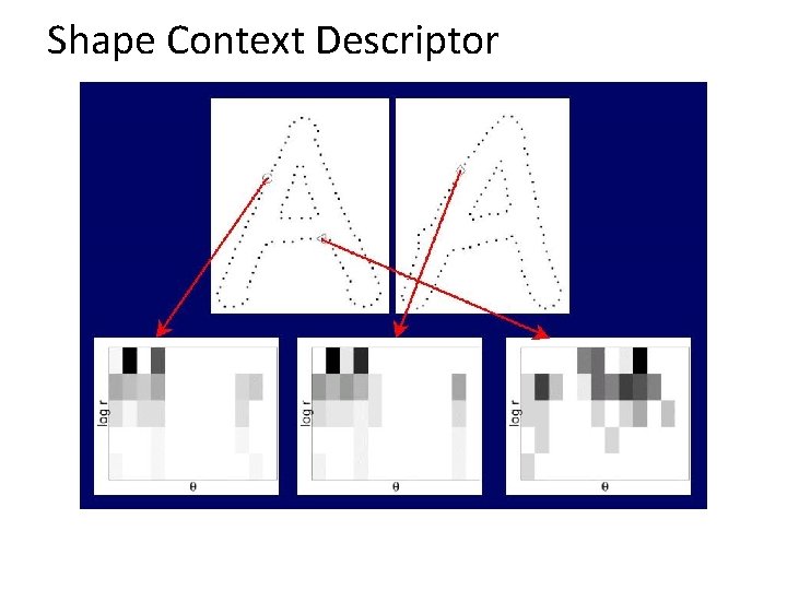
Shape Context Descriptor

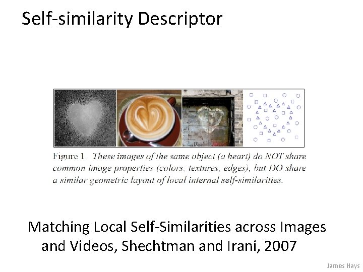
Self-similarity Descriptor Matching Local Self-Similarities across Images and Videos, Shechtman and Irani, 2007 James Hays

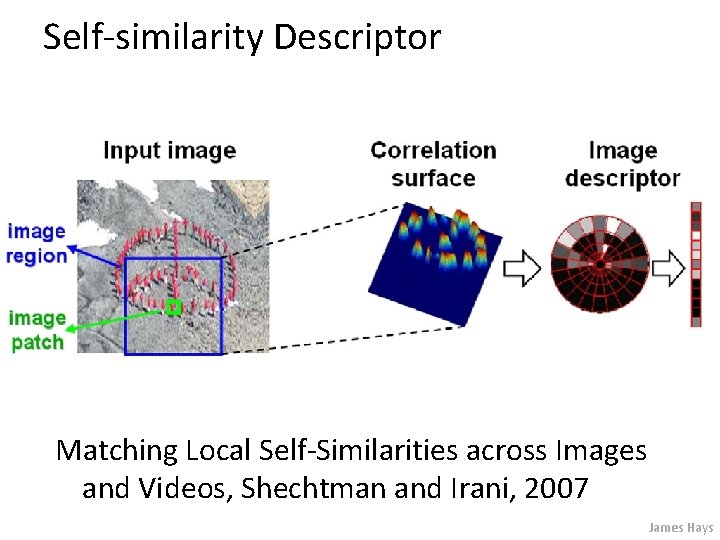
Self-similarity Descriptor Matching Local Self-Similarities across Images and Videos, Shechtman and Irani, 2007 James Hays

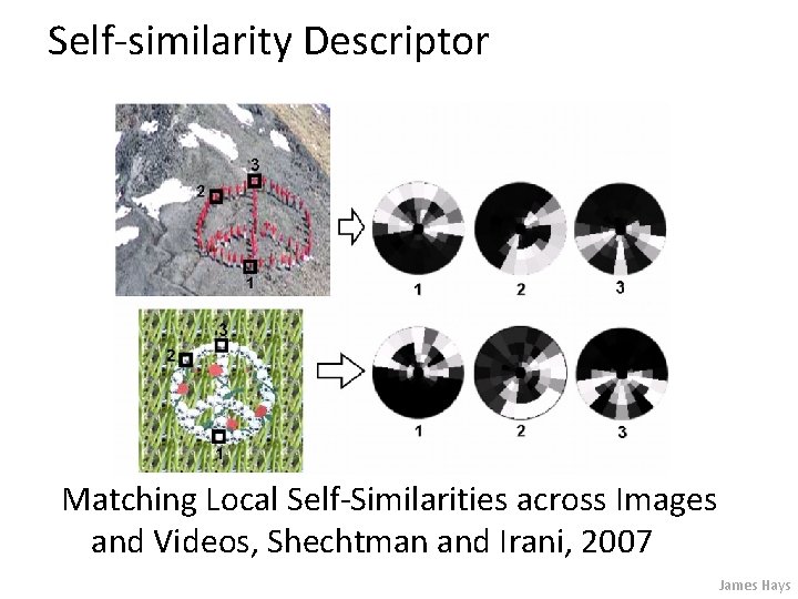
Self-similarity Descriptor Matching Local Self-Similarities across Images and Videos, Shechtman and Irani, 2007 James Hays

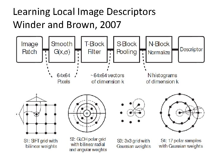
Learning Local Image Descriptors Winder and Brown, 2007

Local Descriptors • Most features can be thought of as templates, histograms (counts), or combinations • The ideal descriptor should be – Robust – Distinctive – Compact – Efficient • Most available descriptors focus on edge/gradient information – Capture texture information – Color rarely used K. Grauman, B. Leibe

Available at a web site near you… • Many local feature detectors have executables available online: – http: //www. robots. ox. ac. uk/~vgg/research/affine – http: //www. cs. ubc. ca/~lowe/keypoints/ – http: //www. vision. ee. ethz. ch/~surf K. Grauman, B. Leibe

Next time • Feature matching, Hough Transform