Lithospheric Layering Outline 1 Receiver Function Method 2

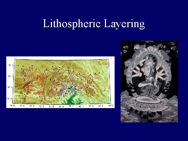
Lithospheric Layering

Outline 1. Receiver Function Method 2. Mapping time to depth (Basic) 3. Advanced applications a. Determining Vp/Vs and Moho depth b. Velocity modeling c. Determining layers of anisotropy and dip

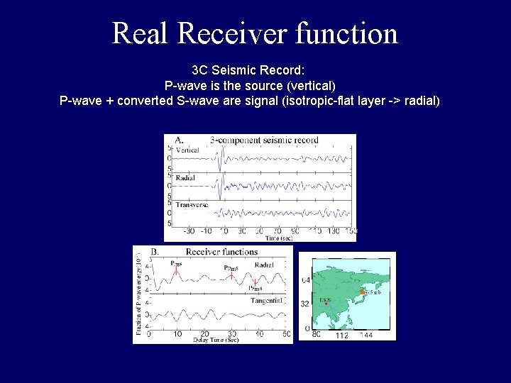
Receiver functions are used to isolate the response function that describes P-wave to S -wave conversions at horizontal velocity interfaces (layers) in the earth below the receiver (hence the name receiver function)

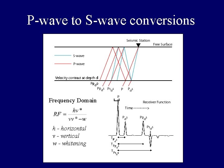
P-wave to S-wave conversions Frequency Domain h - horizontal v - vertical w - whitening �

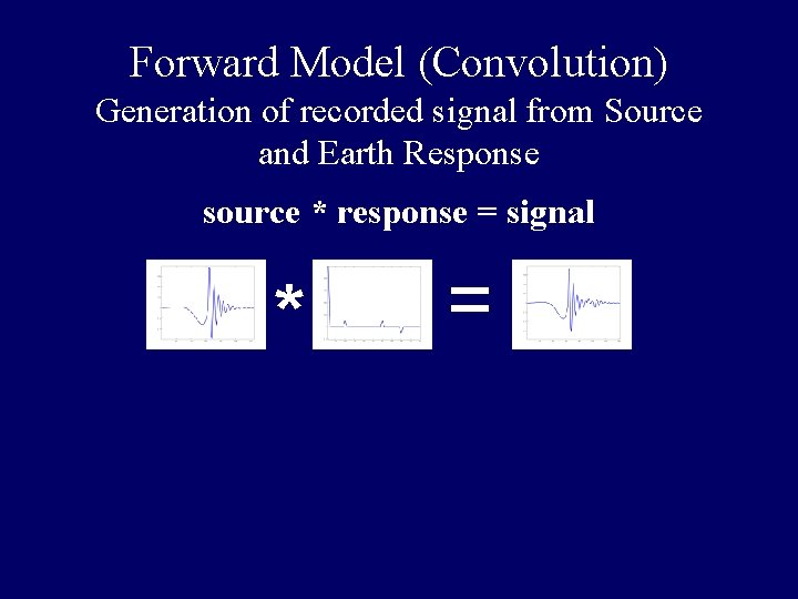
Forward Model (Convolution) Generation of recorded signal from Source and Earth Response source * response = signal * =

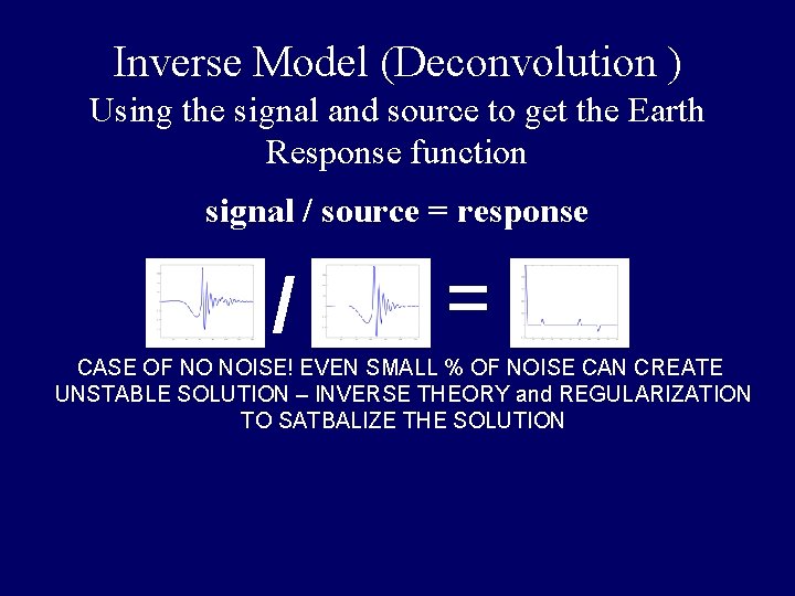
Inverse Model (Deconvolution ) Using the signal and source to get the Earth Response function signal / source = response / = CASE OF NO NOISE! EVEN SMALL % OF NOISE CAN CREATE UNSTABLE SOLUTION – INVERSE THEORY and REGULARIZATION TO SATBALIZE THE SOLUTION

Real Receiver function 3 C Seismic Record: P-wave is the source (vertical) P-wave + converted S-wave are signal (isotropic-flat layer -> radial)

Outline 1. Receiver Function Method 2. Mapping time to depth (Basic) 3. Advanced applications a. Determining Vp/Vs and Moho depth b. Velocity modeling c. Determining layers of anisotropy and dip

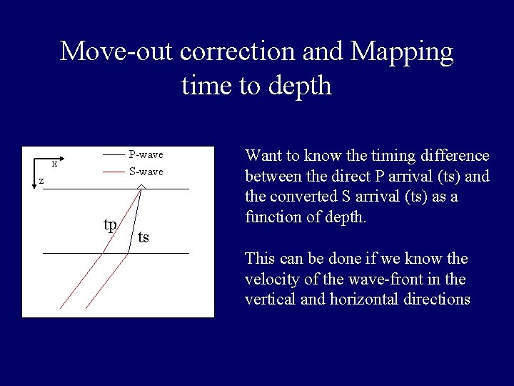
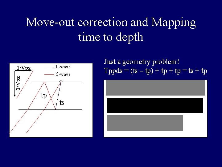
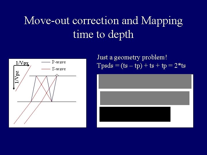
Move-out correction and Mapping time to depth P-wave S-wave x z tp Want to know the timing difference between the direct P arrival (ts) and the converted S arrival (ts) as a function of depth. ts This can be done if we know the velocity of the wave-front in the vertical and horizontal directions

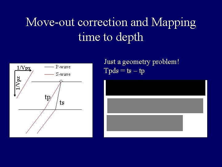
Move-out correction and Mapping time to depth P-wave S-wave 1/Vpz 1/Vpx tp ts Just a geometry problem! Tpds = ts – tp

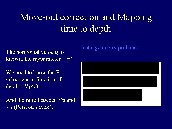
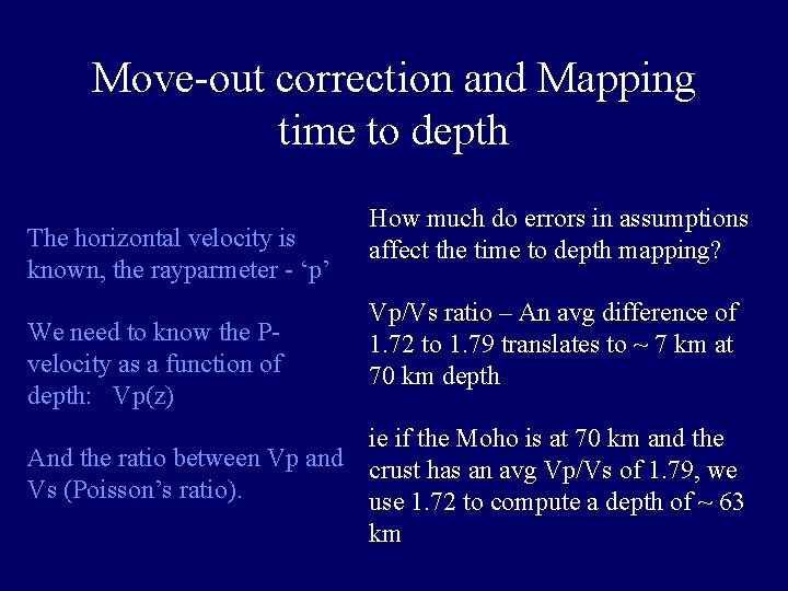
Move-out correction and Mapping time to depth The horizontal velocity is known, the rayparmeter - ‘p’ We need to know the Pvelocity as a function of depth: Vp(z) And the ratio between Vp and Vs (Poisson’s ratio). Just a geometry problem!

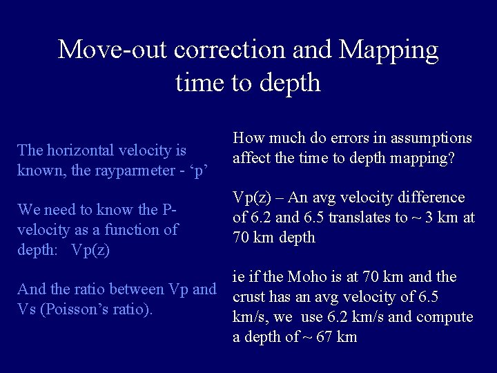
Move-out correction and Mapping time to depth The horizontal velocity is known, the rayparmeter - ‘p’ We need to know the Pvelocity as a function of depth: Vp(z) How much do errors in assumptions affect the time to depth mapping? Vp(z) – An avg velocity difference of 6. 2 and 6. 5 translates to ~ 3 km at 70 km depth ie if the Moho is at 70 km and the And the ratio between Vp and crust has an avg velocity of 6. 5 Vs (Poisson’s ratio). km/s, we use 6. 2 km/s and compute a depth of ~ 67 km

Move-out correction and Mapping time to depth The horizontal velocity is known, the rayparmeter - ‘p’ We need to know the Pvelocity as a function of depth: Vp(z) How much do errors in assumptions affect the time to depth mapping? Vp/Vs ratio – An avg difference of 1. 72 to 1. 79 translates to ~ 7 km at 70 km depth ie if the Moho is at 70 km and the And the ratio between Vp and crust has an avg Vp/Vs of 1. 79, we Vs (Poisson’s ratio). use 1. 72 to compute a depth of ~ 63 km

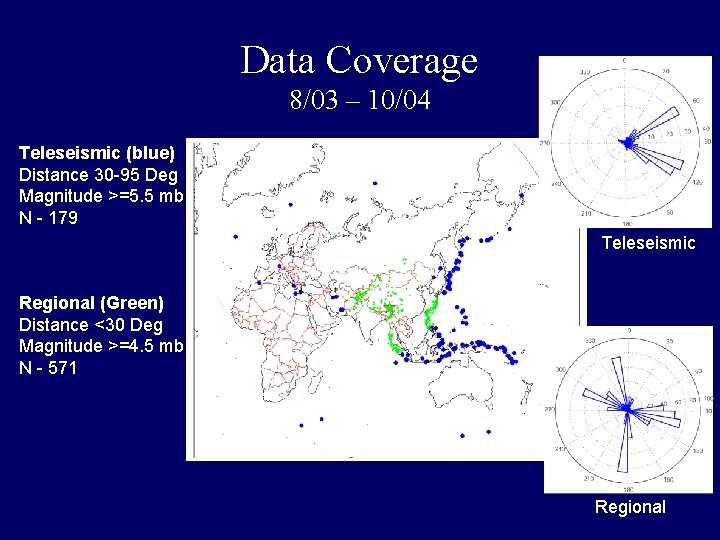
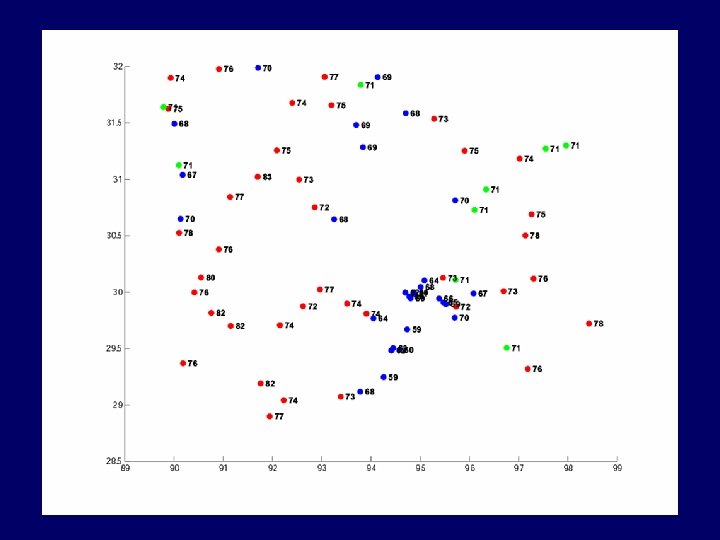
Data Coverage 8/03 – 10/04 Teleseismic (blue) Distance 30 -95 Deg Magnitude >=5. 5 mb N - 179 Teleseismic Regional (Green) Distance <30 Deg Magnitude >=4. 5 mb N - 571 Regional

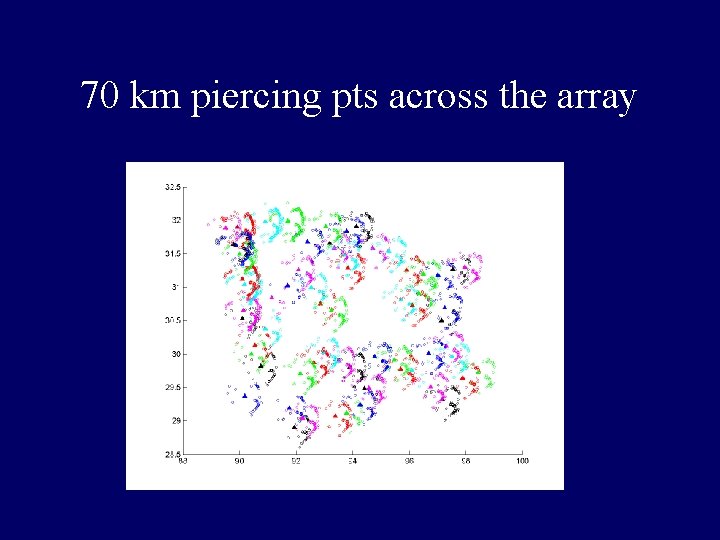
70 km piercing pts across the array

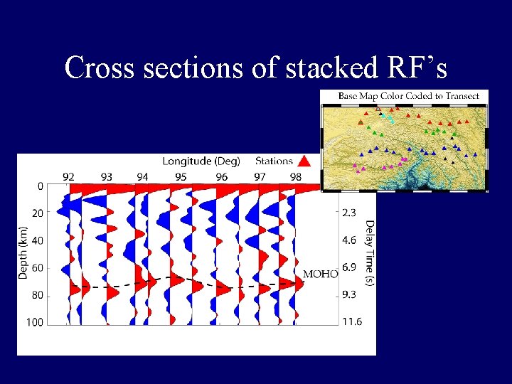
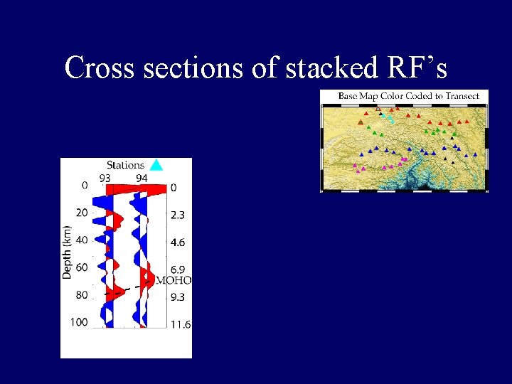
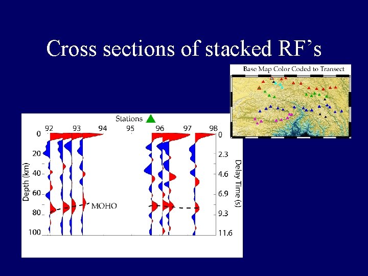
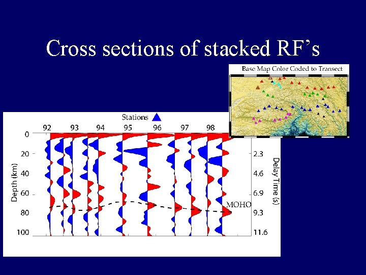
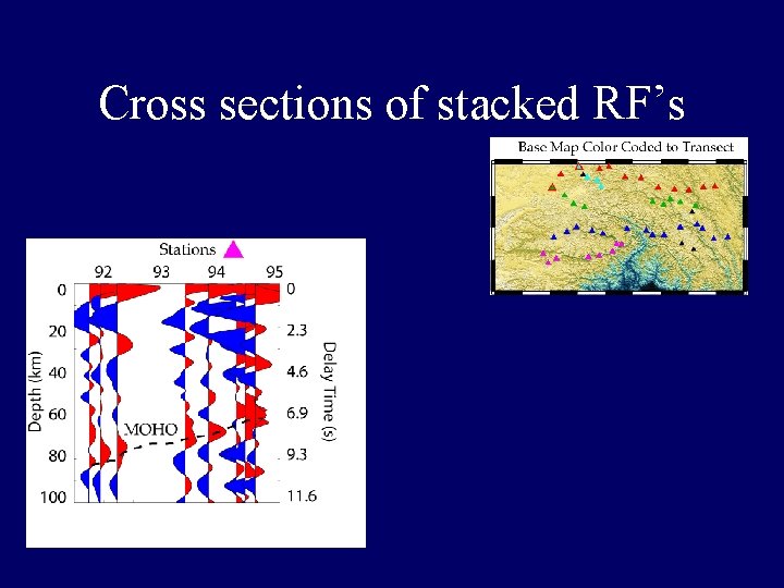
Cross sections of stacked RF’s

Cross sections of stacked RF’s

Cross sections of stacked RF’s

Cross sections of stacked RF’s

Cross sections of stacked RF’s

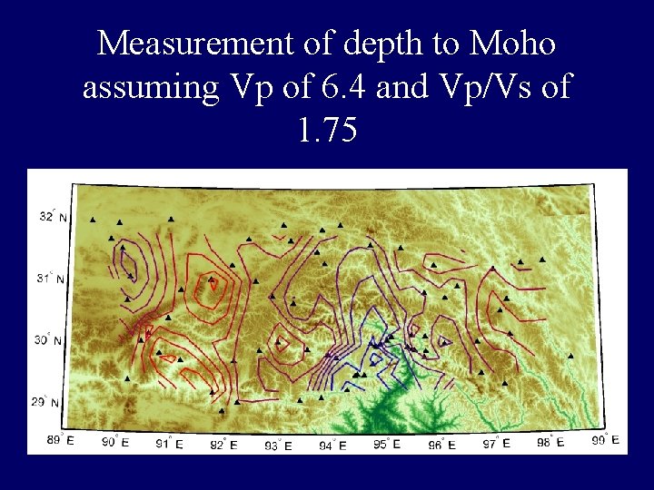
Measurement of depth to Moho assuming Vp of 6. 4 and Vp/Vs of 1. 75

Outline 1. Receiver Function Method 2. Mapping time to depth (Basic) 3. Advanced applications a. Determining Vp/Vs and Moho depth b. Velocity modeling c. Determining layers of anisotropy and dip

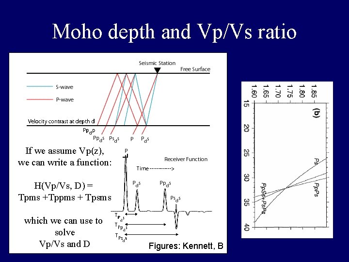
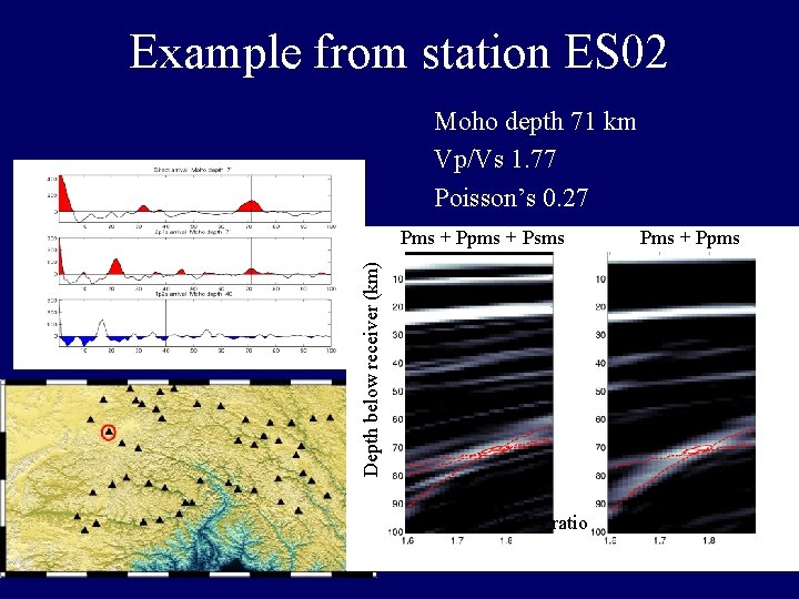
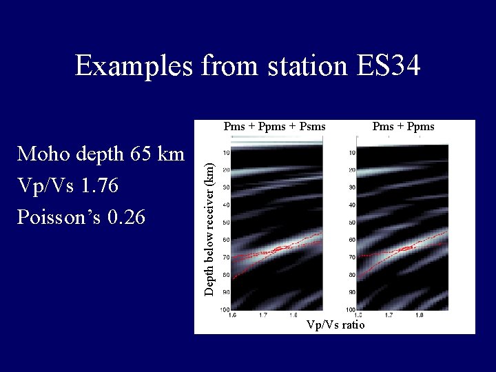
Moho depth and Vp/Vs ratio If we assume Vp(z), we can write a function: � H(Vp/Vs, D) = Tpms +Tppms + Tpsms which we can use to solve Vp/Vs and D Figures: Kennett, B

Example from station ES 02 Moho depth 71 km Vp/Vs 1. 77 Poisson’s 0. 27 Depth below receiver (km) Pms + Ppms + Psms Vp/Vs ratio Pms + Ppms

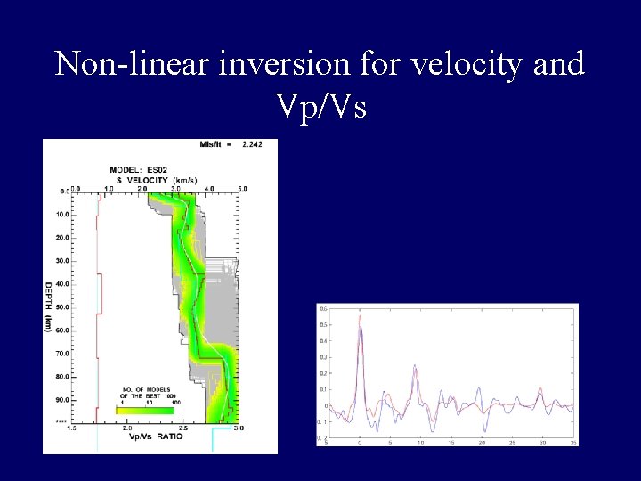
Non-linear inversion for velocity and Vp/Vs

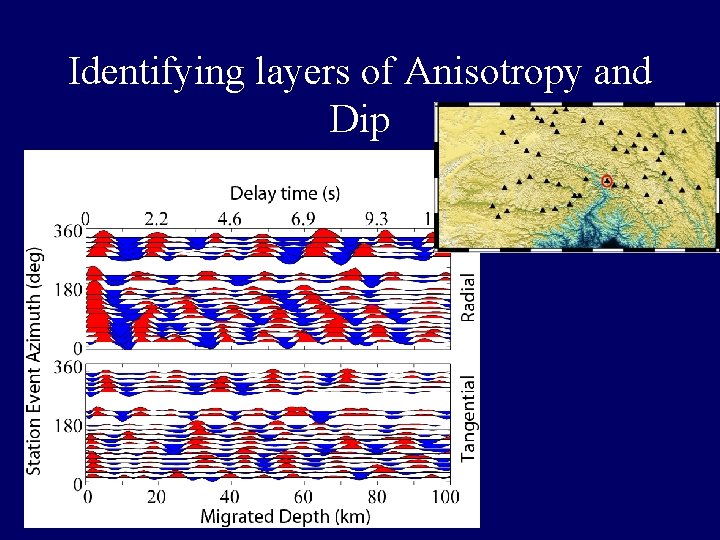
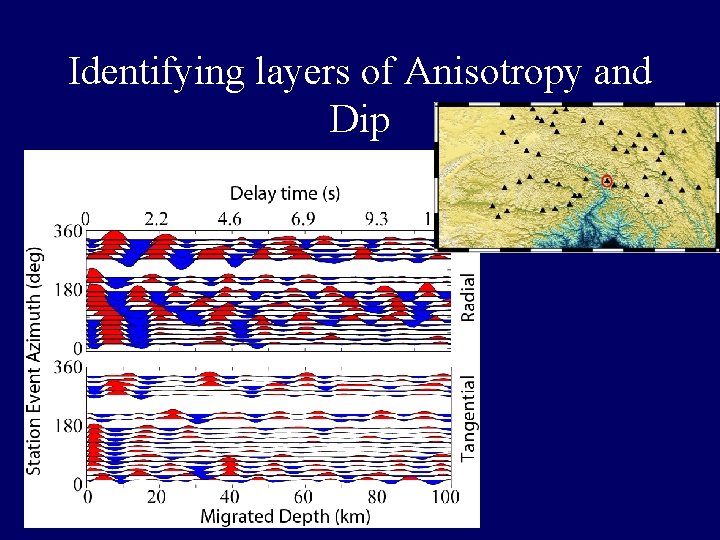
Identifying layers of Anisotropy and Dip

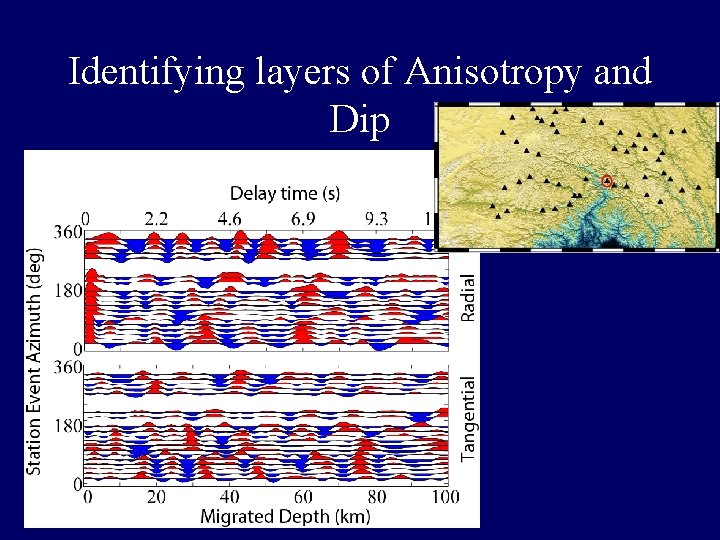
Identifying layers of Anisotropy and Dip

Identifying layers of Anisotropy and Dip

Thank You! The End…

Move-out correction and Mapping time to depth P-wave S-wave 1/Vpz 1/Vpx tp ts Just a geometry problem! Tppds = (ts – tp) + tp = ts + tp

Move-out correction and Mapping time to depth 1/Vpz 1/Vpx P-wave S-wave Just a geometry problem! Tpsds = (ts – tp) + ts + tp = 2*ts

Examples from station ES 34 Moho depth 65 km Vp/Vs 1. 76 Poisson’s 0. 26 Depth below receiver (km) Pms + Ppms + Psms Vp/Vs ratio Pms + Ppms