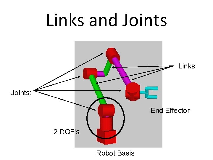
Links and Joints Links and Joints Links Joints




- Slides: 42

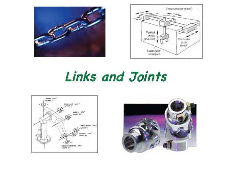
Links and Joints

Links and Joints Links Joints: End Effector 2 DOF’s Robot Basis


Denavit – Hartenberg details and examples

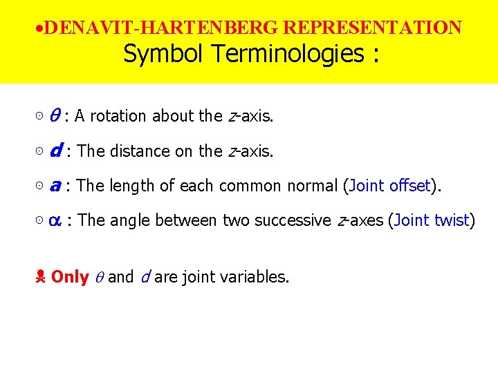
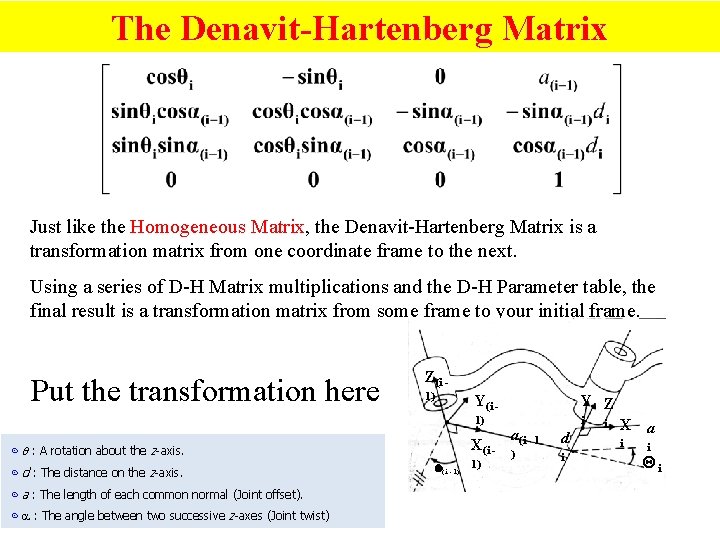
·DENAVIT-HARTENBERG REPRESENTATION Chapter 2 Symbol Terminologies : Robot Kinematics: Position Analysis ⊙ : A rotation about the z-axis. ⊙ d : The distance on the z-axis. ⊙ a : The length of each common normal (Joint offset). ⊙ : The angle between two successive z-axes (Joint twist) Only and d are joint variables.

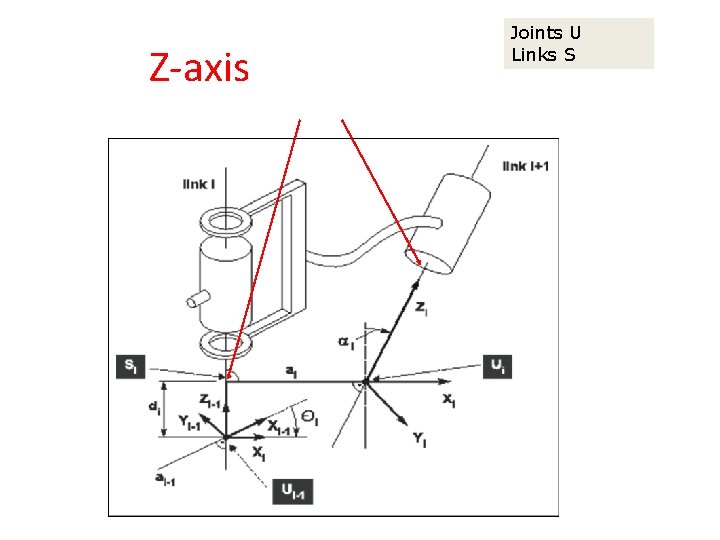
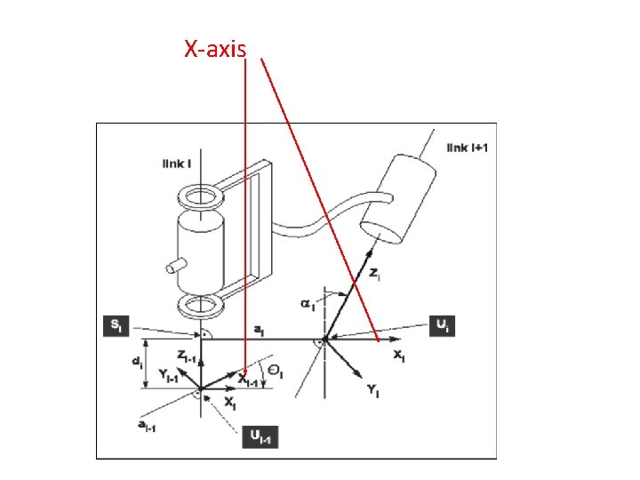
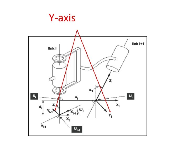
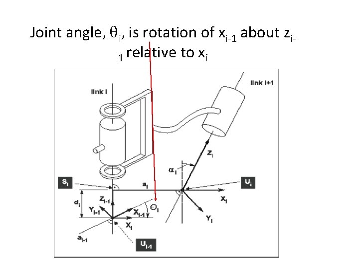
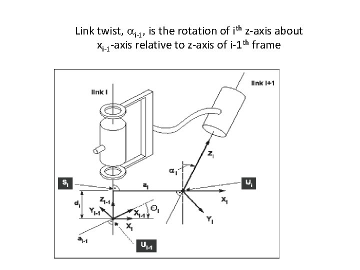
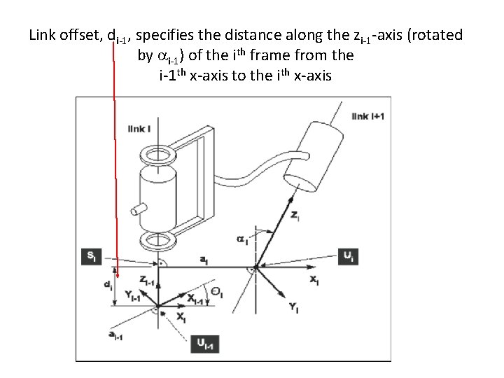
Joints U Links S Z-axis aligned with joint

X-axis aligned with outgoing limb

Y-axis is orthogonal

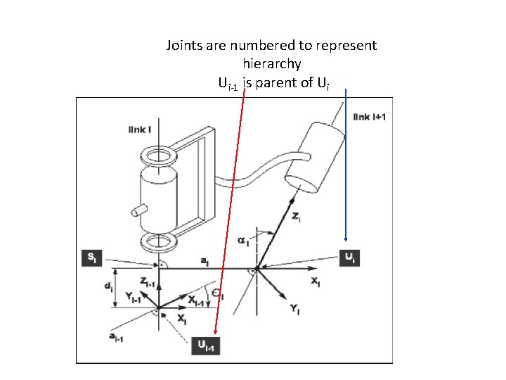
Joints are numbered to represent hierarchy Ui-1 is parent of Ui

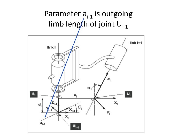
Parameter ai-1 is outgoing limb length of joint Ui-1

Joint angle, qi, is rotation of xi-1 about zi 1 relative to xi

Link twist, i-1, is the rotation of ith z-axis about xi-1 -axis relative to z-axis of i-1 th frame

Link offset, di-1, specifies the distance along the zi-1 -axis (rotated by i-1) of the ith frame from the i-1 th x-axis to the ith x-axis

DENAVIT-HARTENBERG REPRESENTATION PROCEDURES Start point: • Assign joint number n to the first shown joint. • Assign a local reference frame for each and every joint before or after these joints. • Y-axis is not used in D-H representation.

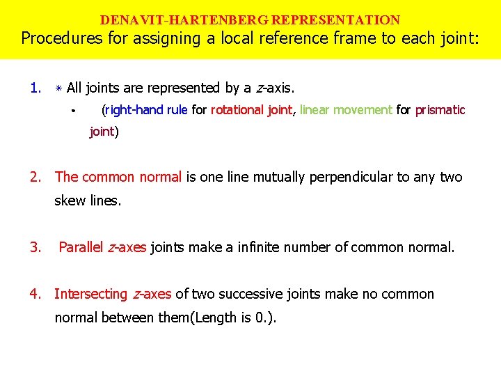
DENAVIT-HARTENBERG REPRESENTATION Procedures for assigning a local reference frame to each joint: 1. ٭ All joints are represented by a z-axis. ● (right-hand rule for rotational joint, linear movement for prismatic joint) 2. The common normal is one line mutually perpendicular to any two skew lines. 3. Parallel z-axes joints make a infinite number of common normal. 4. Intersecting z-axes of two successive joints make no common normal between them(Length is 0. ).

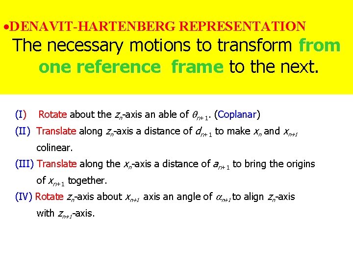
·DENAVIT-HARTENBERG Chapter. REPRESENTATION 2 Robot Kinematics: Positionto Analysis The necessary motions transform from one reference frame to the next. (I) Rotate about the zn-axis an able of n+1. (Coplanar) (II) Translate along zn-axis a distance of dn+1 to make xn and xn+1 colinear. (III) Translate along the xn-axis a distance of an+1 to bring the origins of xn+1 together. (IV) Rotate zn-axis about xn+1 axis an angle of n+1 to align zn-axis with zn+1 -axis.

Denavit Hartenberg Parameters – a general explanation

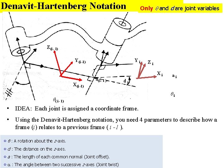
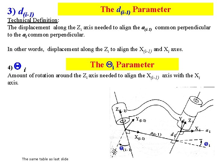
Denavit-Hartenberg Notation Only and d are joint variables Z(i - 1) Y(i -1) X(i -1) Yi a(i - 1 ) Zi Xi di ai i ( i - 1) • IDEA: Each joint is assigned a coordinate frame. • Using the Denavit-Hartenberg notation, you need 4 parameters to describe how a frame (i) relates to a previous frame ( i -1 ). ⊙ • : ATHE rotation about the z-axis. PARAMETERS/VARIABLES: ⊙ d : The distance on the z-axis. ⊙ a : The length of each common normal (Joint offset). ⊙ : The angle between two successive z-axes (Joint twist) � , a , d, �

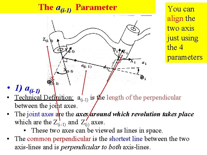
The a(i-1) Parameter Z(i - 1) Y(i -1) X(i -1) • 1) a(i-1) ( i - 1) Yi a(i - 1 ) Zi Xi di ai You can align the two axis just using the 4 parameters i • Technical Definition: a(i-1) is the length of the perpendicular between the joint axes. • The joint axes are the axes around which revolution takes place which are the Z(i-1) and Z(i) axes. • These two axes can be viewed as lines in space. • The common perpendicular is the shortest line between the two axis-lines and is perpendicular to both axis-lines.

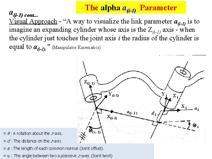
a(i-1) cont. . . The alpha a(i-1) Parameter Visual Approach - “A way to visualize the link parameter a(i-1) is to imagine an expanding cylinder whose axis is the Z(i-1) axis - when the cylinder just touches the joint axis i the radius of the cylinder is equal to a(i-1). ” (Manipulator Kinematics) Z(i - 1) Y(i -1) X(i -1) ⊙ : A rotation about the z-axis. ( i - 1) ⊙ d : The distance on the z-axis. ⊙ a : The length of each common normal (Joint offset). ⊙ : The angle between two successive z-axes (Joint twist) Yi a(i - 1 ) Zi Xi di ai i

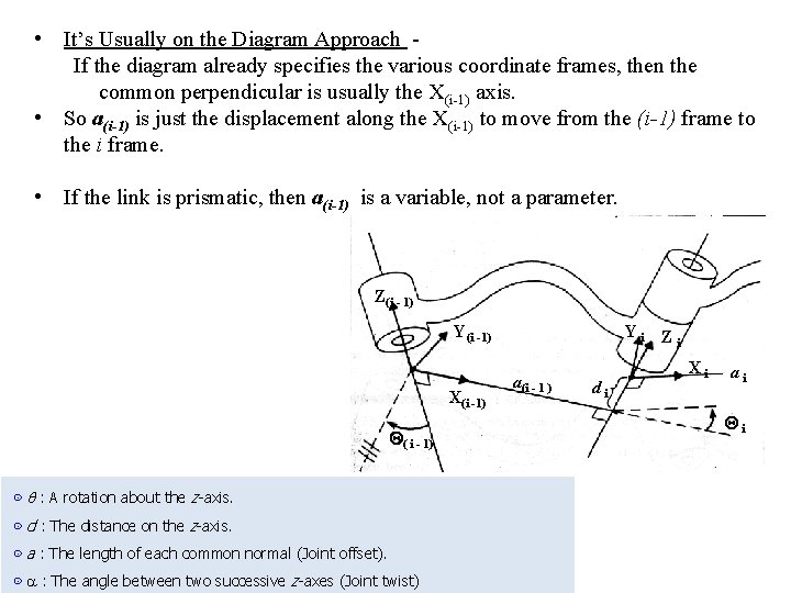
• It’s Usually on the Diagram Approach If the diagram already specifies the various coordinate frames, then the common perpendicular is usually the X(i-1) axis. • So a(i-1) is just the displacement along the X(i-1) to move from the (i-1) frame to the i frame. • If the link is prismatic, then a(i-1) is a variable, not a parameter. Z(i - 1) Y(i -1) X(i -1) ( i - 1) ⊙ : A rotation about the z-axis. ⊙ d : The distance on the z-axis. ⊙ a : The length of each common normal (Joint offset). ⊙ : The angle between two successive z-axes (Joint twist) Yi a(i - 1 ) di Zi Xi ai i

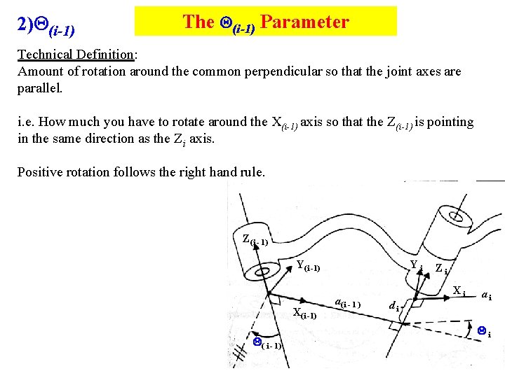
2) (i-1) The (i-1) Parameter Technical Definition: Amount of rotation around the common perpendicular so that the joint axes are parallel. i. e. How much you have to rotate around the X(i-1) axis so that the Z(i-1) is pointing in the same direction as the Zi axis. Positive rotation follows the right hand rule. Z(i - 1) Y(i -1) X(i -1) ( i - 1) Yi a(i - 1 ) Zi Xi di ai i

3) d(i-1) The d(i-1) Parameter Technical Definition: The displacement along the Zi axis needed to align the a(i-1) common perpendicular to the ai common perpendicular. In other words, displacement along the Zi to align the X(i-1) and Xi axes. The i Parameter 4) i Amount of rotation around the Zi axis needed to align the X(i-1) axis with the Xi axis. Z(i - 1) Y(i -1) X(i -1) ( i - 1) The same table as last slide Yi Z i a(i - 1 ) di Xi ai i

The Denavit-Hartenberg Matrix Just like the Homogeneous Matrix, the Denavit-Hartenberg Matrix is a transformation matrix from one coordinate frame to the next. Using a series of D-H Matrix multiplications and the D-H Parameter table, the final result is a transformation matrix from some frame to your initial frame. Put the transformation here Z(i 1) ⊙ a : The length of each common normal (Joint offset). ⊙ : The angle between two successive z-axes (Joint twist) Y Z 1) i X(i - ⊙ : A rotation about the z-axis. ⊙ d : The distance on the z-axis. Y(i - ( i - 1) 1) a(i - 1 d ) i i X a i i i

Example: Calculating the final DH matrix with the DH Parameter Table

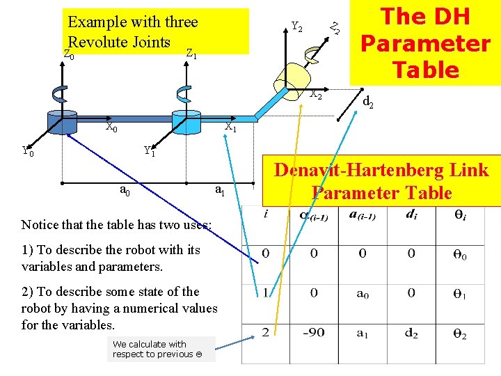
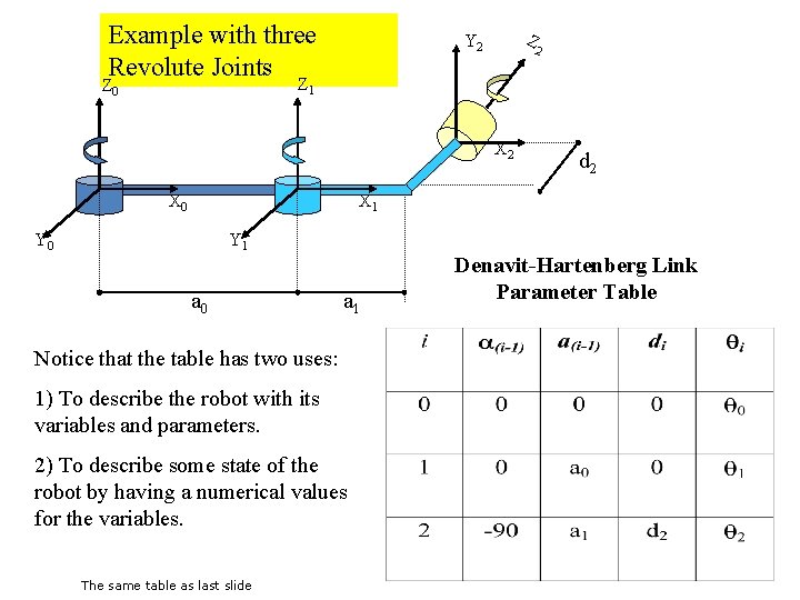
Example with three Revolute Joints Z Y 2 2 Z 1 Z 0 X 2 X 0 The DH Parameter Table d 2 X 1 Y 0 Y 1 a 0 a 1 Notice that the table has two uses: 1) To describe the robot with its variables and parameters. 2) To describe some state of the robot by having a numerical values for the variables. We calculate with respect to previous Denavit-Hartenberg Link Parameter Table

Example with three Revolute Joints Z Y 2 2 Z 1 Z 0 X 2 X 0 d 2 X 1 Y 0 Y 1 a 0 a 1 Notice that the table has two uses: 1) To describe the robot with its variables and parameters. 2) To describe some state of the robot by having a numerical values for the variables. The same table as last slide Denavit-Hartenberg Link Parameter Table

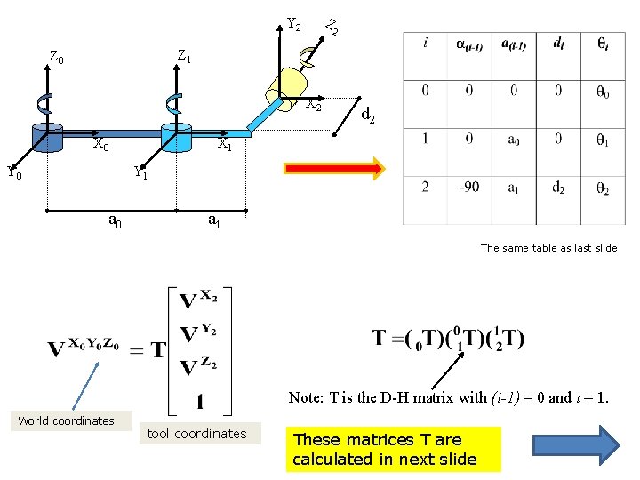
Z Y 2 2 Z 1 Z 0 X 2 X 0 d 2 X 1 Y 0 Y 1 a 0 a 1 The same table as last slide Note: T is the D-H matrix with (i-1) = 0 and i = 1. World coordinates tool coordinates These matrices T are calculated in next slide

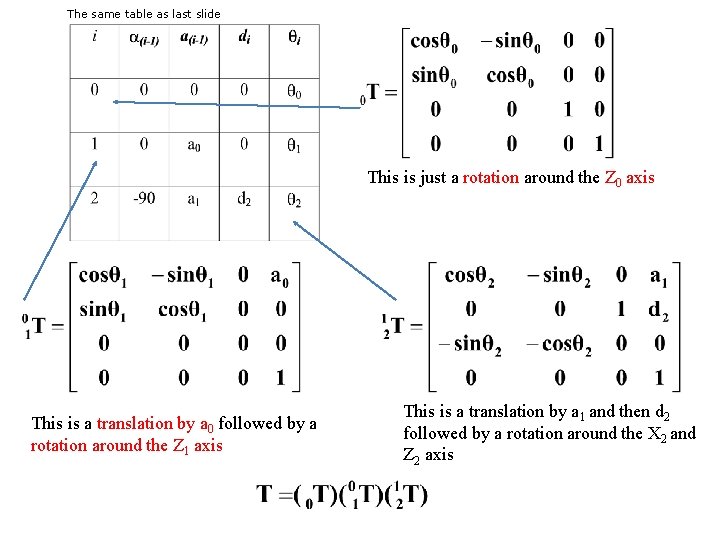
The same table as last slide This is just a rotation around the Z 0 axis This is a translation by a 0 followed by a rotation around the Z 1 axis This is a translation by a 1 and then d 2 followed by a rotation around the X 2 and Z 2 axis

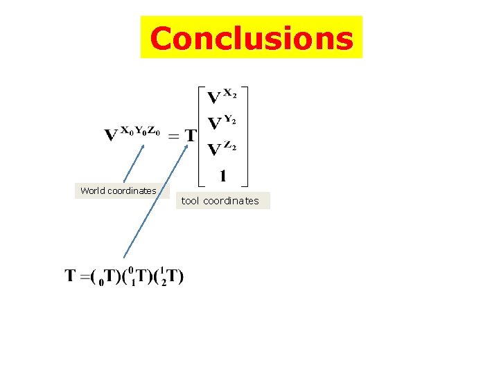
Conclusions World coordinates tool coordinates

Forward Kinematics

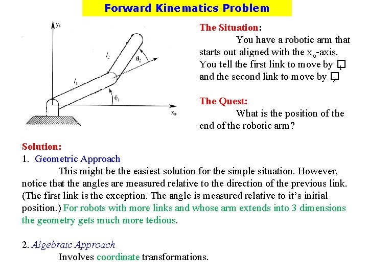
Forward Kinematics Problem The Situation: You have a robotic arm that starts out aligned with the xo-axis. You tell the first link to move by � 1 and the second link to move by � 2. The Quest: What is the position of the end of the robotic arm? Solution: 1. Geometric Approach This might be the easiest solution for the simple situation. However, notice that the angles are measured relative to the direction of the previous link. (The first link is the exception. The angle is measured relative to it’s initial position. ) For robots with more links and whose arm extends into 3 dimensions the geometry gets much more tedious 2. Algebraic Approach Involves coordinate transformations.

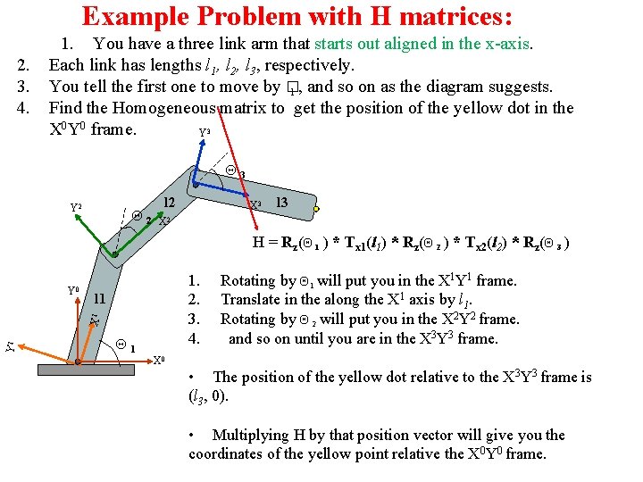
Example Problem with H matrices: 2. 3. 4. 1. You have a three link arm that starts out aligned in the x-axis. Each link has lengths l 1, l 2, l 3, respectively. You tell the first one to move by � 1 , and so on as the diagram suggests. Find the Homogeneous matrix to get the position of the yellow dot in the X 0 Y 0 frame. Y 3 3 Y 2 2 l 2 X 3 l 3 X 2 H = Rz( 1 ) * Tx 1(l 1) * Rz( 2 ) * Tx 2(l 2) * Rz( 3 ) 1. 2. 3. 4. l 1 Y 1 X 1 Y 0 1 Rotating by 1 will put you in the X 1 Y 1 frame. Translate in the along the X 1 axis by l 1. Rotating by 2 will put you in the X 2 Y 2 frame. and so on until you are in the X 3 Y 3 frame. X 0 • The position of the yellow dot relative to the X 3 Y 3 frame is (l 3, 0). • Multiplying H by that position vector will give you the coordinates of the yellow point relative the X 0 Y 0 frame.

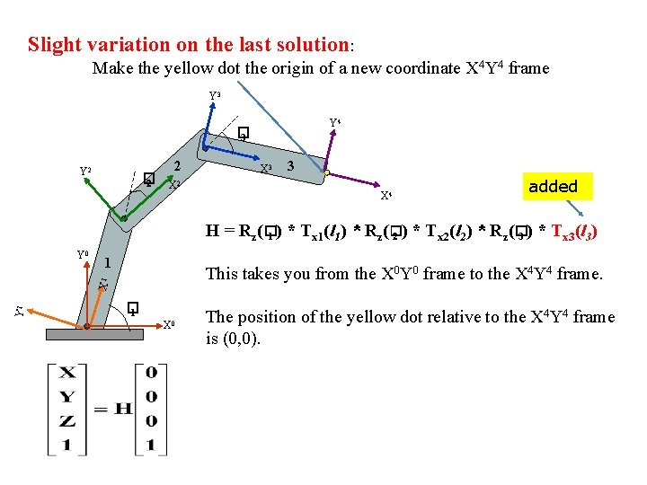
Slight variation on the last solution: Make the yellow dot the origin of a new coordinate X 4 Y 4 frame Y 3 Y 4 � 3 Y 2 � 2 2 X 3 3 X 4 added H = R z (� 1 ) * Tx 1(l 1) * Rz(� 2 ) * Tx 2(l 2) * Rz(� 3 ) * Tx 3(l 3) 1 This takes you from the X 0 Y 0 frame to the X 4 Y 4 frame. Y 1 X 1 Y 0 � 1 X 0 The position of the yellow dot relative to the X 4 Y 4 frame is (0, 0).

THE INVERSE KINEMATIC SOLUTION OF A ROBOT

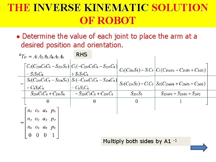
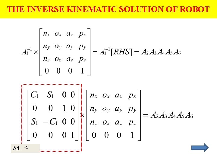
THE INVERSE KINEMATIC SOLUTION OF ROBOT · Determine the value of each joint to place the arm at a desired position and orientation. RHS Multiply both sides by A 1 -1

THE INVERSE KINEMATIC SOLUTION OF ROBOT A 1 -1

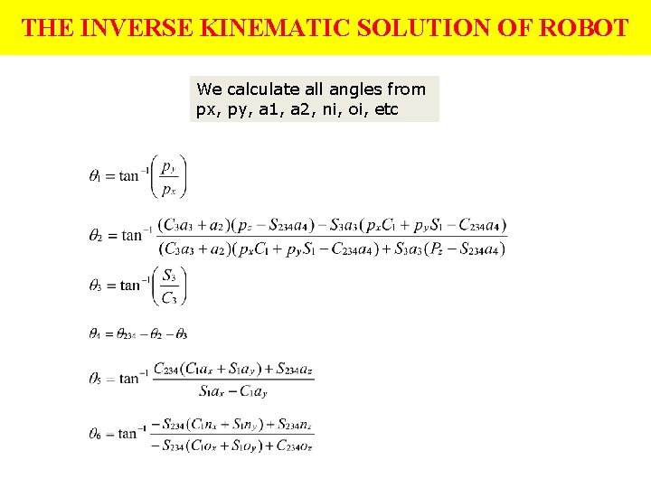
THE INVERSE KINEMATIC SOLUTION OF ROBOT We calculate all angles from px, py, a 1, a 2, ni, oi, etc

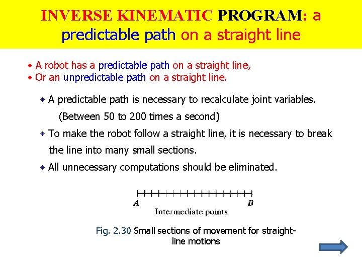
INVERSE KINEMATIC PROGRAM: a predictable path on a straight line · A robot has a predictable path on a straight line, · Or an unpredictable path on a straight line. ٭ A predictable path is necessary to recalculate joint variables. (Between 50 to 200 times a second) ٭ To make the robot follow a straight line, it is necessary to break the line into many small sections. ٭ All unnecessary computations should be eliminated. Fig. 2. 30 Small sections of movement for straightline motions

PROBLEMS with DH

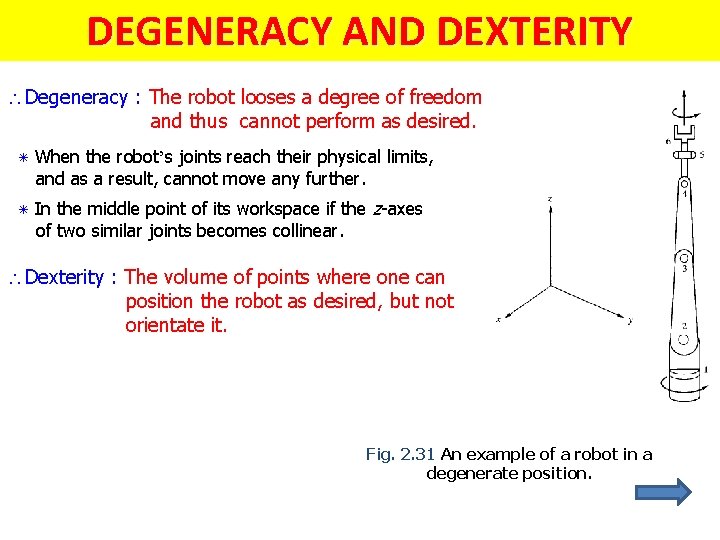
DEGENERACY AND DEXTERITY Degeneracy : The robot looses a degree of freedom and thus cannot perform as desired. ٭ When the robot’s joints reach their physical limits, and as a result, cannot move any further. ٭ In the middle point of its workspace if the z-axes of two similar joints becomes collinear. Dexterity : The volume of points where one can position the robot as desired, but not orientate it. Fig. 2. 31 An example of a robot in a degenerate position.

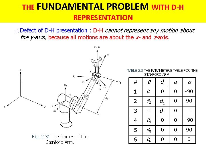
THE FUNDAMENTAL PROBLEM WITH D-H REPRESENTATION Defect of D-H presentation : D-H cannot represent any motion about the y-axis, because all motions are about the x- and z-axis. TABLE 2. 3 THE PARAMETERS TABLE FOR THE STANFORD ARM Fig. 2. 31 The frames of the Stanford Arm. # d a 1 1 0 0 -90 2 2 d 1 0 90 3 0 d 1 0 0 4 4 0 0 -90 5 5 0 0 90 6 6 0 0 0