Linkage Genetic Mapping in Eukaryotes 1 LINKAGE AND

Linkage & Genetic Mapping in Eukaryotes 1

LINKAGE AND CROSSING OVER �In eukaryotic species, each linear chromosome contains a long piece of DNA – A typical chromosome contains many hundred or even a few thousand different genes �The term linkage has two related meanings – 1. Two or more genes can be located on the same chromosome – 2. Genes that are close together tend to be transmitted as a unit Copyright ©The Mc. Graw-Hill Companies, Inc. Permission required for reproduction or display 2

Linkage Groups �Chromosomes are called linkage groups – They contain a group of genes that are linked together �The number of linkage groups is the number of types of chromosomes of the species – For example, in humans � 22 autosomal linkage groups �An X chromosome linkage group �A Y chromosome linkage group �Genes that are far apart on the same chromosome can independently assort from each other – This is due to crossing-over or recombination Copyright ©The Mc. Graw-Hill Companies, Inc. Permission required for reproduction or display 3

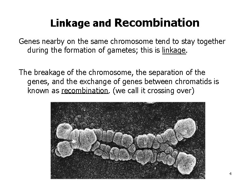
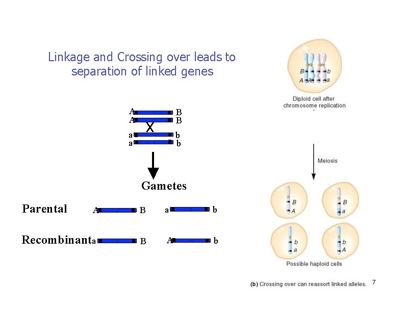
Linkage and Recombination Genes nearby on the same chromosome tend to stay together during the formation of gametes; this is linkage. The breakage of the chromosome, the separation of the genes, and the exchange of genes between chromatids is known as recombination. (we call it crossing over) 4

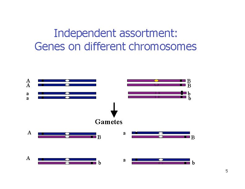
Independent assortment: Genes on different chromosomes A A a a B B b b Gametes A A B b a a B b 5

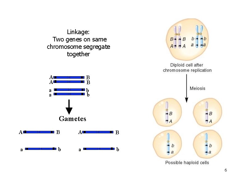
Linkage: Two genes on same chromosome segregate together A A a a B B b b Gametes A B a b 6

Linkage and Crossing over leads to separation of linked genes A A a a B B x b b Gametes Parental A Recombinanta B a b B A b 7

Crossing Over Can Produce Recombinant Phenotypes �In diploid eukaryotic species – linkage can be altered during meiosis as a result of crossing over (recombination) �Crossing over – Occurs during prophase I of meiosis – Non-sister chromatids of homologous chromosomes exchange DNA segments Copyright ©The Mc. Graw-Hill Companies, Inc. Permission required for reproduction or display 8

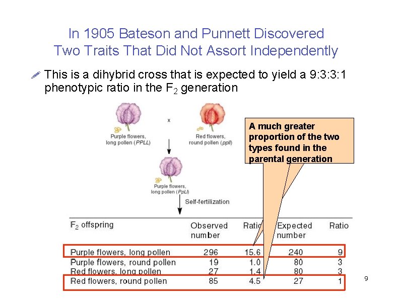
In 1905 Bateson and Punnett Discovered Two Traits That Did Not Assort Independently This is a dihybrid cross that is expected to yield a 9: 3: 3: 1 phenotypic ratio in the F 2 generation A much greater proportion of the two types found in the parental generation Copyright ©The Mc. Graw-Hill Companies, Inc. Permission required for reproduction or display 9

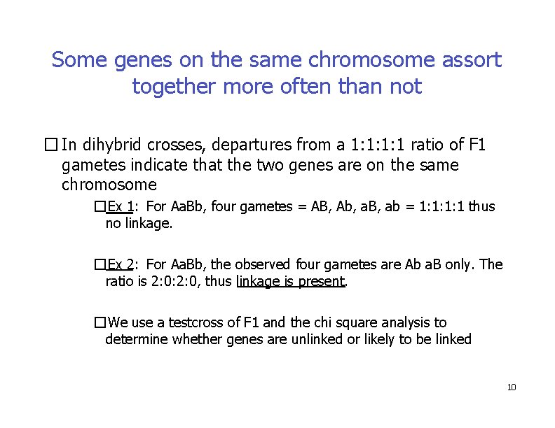
Some genes on the same chromosome assort together more often than not � In dihybrid crosses, departures from a 1: 1: 1: 1 ratio of F 1 gametes indicate that the two genes are on the same chromosome �Ex 1: For Aa. Bb, four gametes = AB, Ab, a. B, ab = 1: 1: 1: 1 thus no linkage. �Ex 2: For Aa. Bb, the observed four gametes are Ab a. B only. The ratio is 2: 0: 2: 0, thus linkage is present. �We use a testcross of F 1 and the chi square analysis to determine whether genes are unlinked or likely to be linked 10

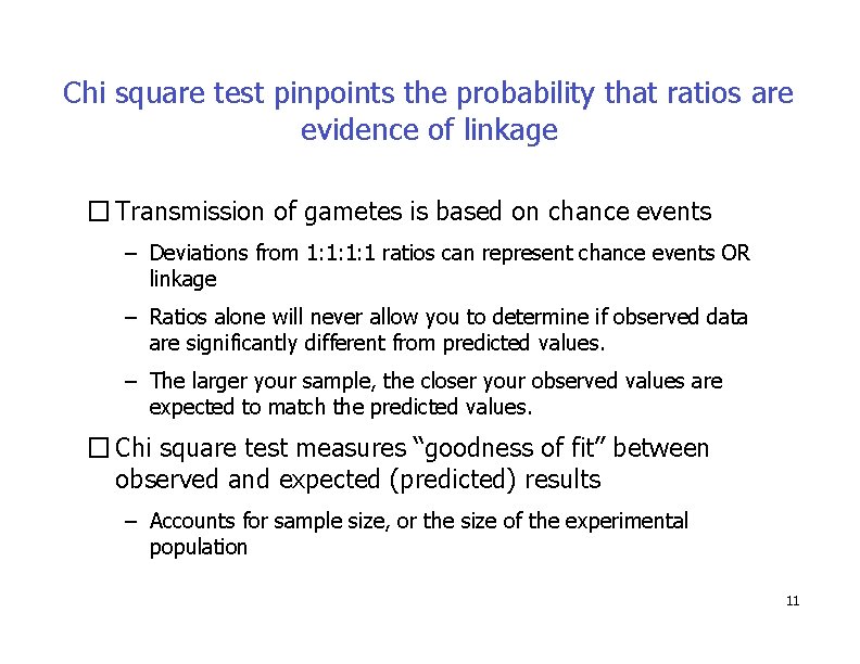
Chi square test pinpoints the probability that ratios are evidence of linkage � Transmission of gametes is based on chance events – Deviations from 1: 1: 1: 1 ratios can represent chance events OR linkage – Ratios alone will never allow you to determine if observed data are significantly different from predicted values. – The larger your sample, the closer your observed values are expected to match the predicted values. � Chi square test measures “goodness of fit” between observed and expected (predicted) results – Accounts for sample size, or the size of the experimental population 11

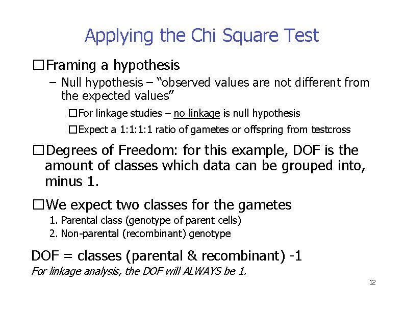
Applying the Chi Square Test �Framing a hypothesis – Null hypothesis – “observed values are not different from the expected values” �For linkage studies – no linkage is null hypothesis �Expect a 1: 1: 1: 1 ratio of gametes or offspring from testcross �Degrees of Freedom: for this example, DOF is the amount of classes which data can be grouped into, minus 1. �We expect two classes for the gametes 1. Parental class (genotype of parent cells) 2. Non-parental (recombinant) genotype DOF = classes (parental & recombinant) -1 For linkage analysis, the DOF will ALWAYS be 1. 12

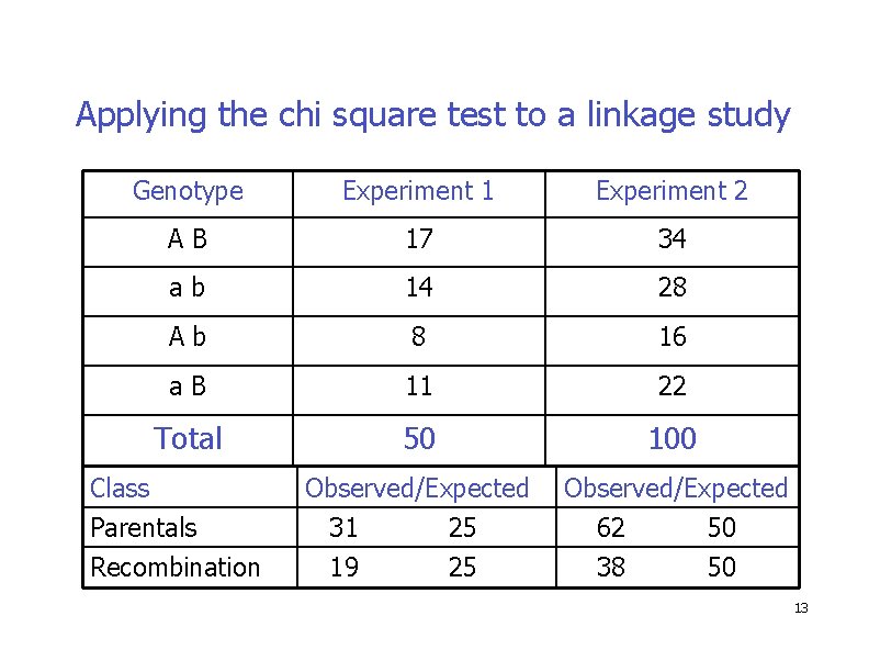
Applying the chi square test to a linkage study Genotype Experiment 1 Experiment 2 AB 17 34 ab 14 28 Ab 8 16 a. B 11 22 Total 50 100 Observed/Expected Class Parentals Recombination 31 19 25 25 62 38 50 50 13

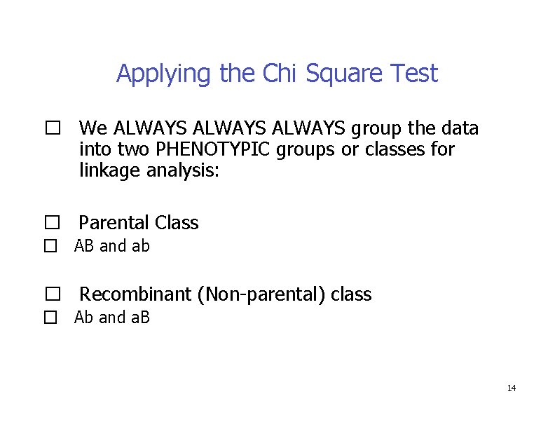
Applying the Chi Square Test � We ALWAYS group the data into two PHENOTYPIC groups or classes for linkage analysis: � Parental Class � AB and ab � Recombinant (Non-parental) class � Ab and a. B 14

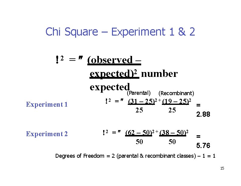
Chi Square – Experiment 1 & 2 2 = (observed – expected)2 number expected(Parental) (Recombinant) Experiment 1 Experiment 2 2 = (31 – 25)2 + (19 – 25)2 = 25 25 2. 88 2 = (62 – 50)2 + (38 – 50)2 50 50 = 5. 76 Degrees of Freedom = 2 (parental & recombinant classes) – 1 = 1 15

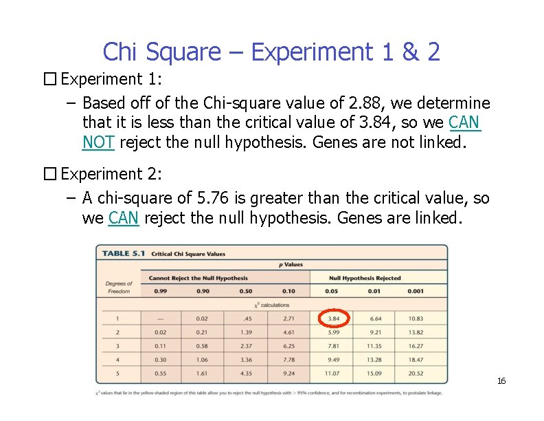
Chi Square – Experiment 1 & 2 � Experiment 1: – Based off of the Chi-square value of 2. 88, we determine that it is less than the critical value of 3. 84, so we CAN NOT reject the null hypothesis. Genes are not linked. � Experiment 2: – A chi-square of 5. 76 is greater than the critical value, so we CAN reject the null hypothesis. Genes are linked. 16

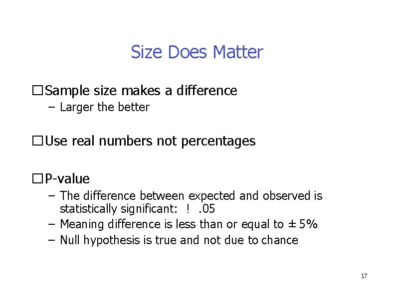
Size Does Matter �Sample size makes a difference – Larger the better �Use real numbers not percentages �P-value – The difference between expected and observed is statistically significant: !. 05 – Meaning difference is less than or equal to ± 5% – Null hypothesis is true and not due to chance 17

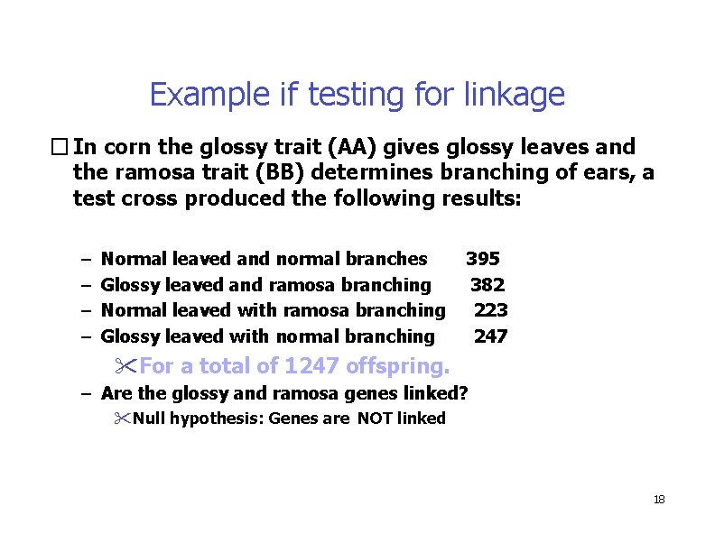
Example if testing for linkage � In corn the glossy trait (AA) gives glossy leaves and the ramosa trait (BB) determines branching of ears, a test cross produced the following results: – – Normal leaved and normal branches Glossy leaved and ramosa branching Normal leaved with ramosa branching Glossy leaved with normal branching 395 382 223 247 For a total of 1247 offspring. – Are the glossy and ramosa genes linked? Null hypothesis: Genes are NOT linked 18

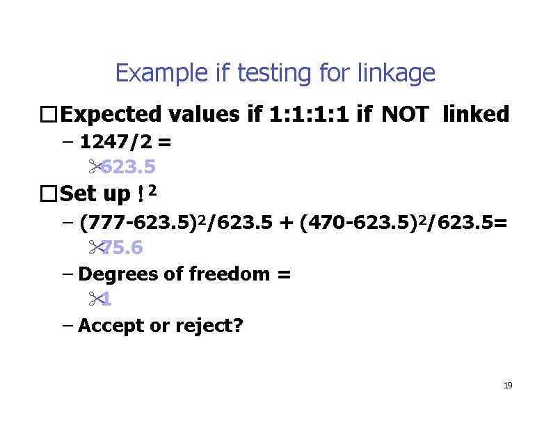
Example if testing for linkage �Expected values if 1: 1: 1: 1 if NOT linked – 1247/2 = 623. 5 �Set up 2 – (777 -623. 5)2/623. 5 + (470 -623. 5)2/623. 5= 75. 6 – Degrees of freedom = 1 – Accept or reject? 19

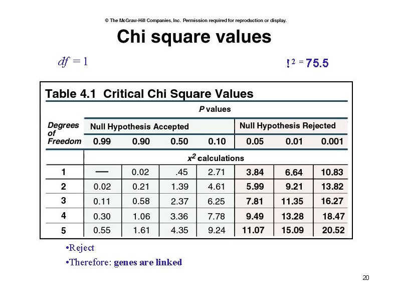
df = 1 2 = 75. 5 • Reject • Therefore: genes are linked 20

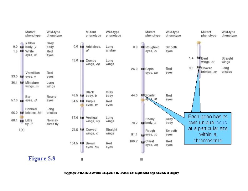
GENETIC MAPPING IN PLANTS AND ANIMALS �Genetic mapping is also known as gene mapping or chromosome mapping �Its purpose is to determine the linear order of linked genes along the same chromosome �Figure 5. 8 illustrates a simplified genetic linkage map of Drosophila melanogaster Copyright ©The Mc. Graw-Hill Companies, Inc. Permission required for reproduction or display

Each gene has its own unique locus at a particular site within a chromosome Figure 5. 8 Copyright ©The Mc. Graw-Hill Companies, Inc. Permission required for reproduction or display

Genetic Maps �Genetic maps are useful in many ways: they – 1. allow us to understand the overall complexity and genetic organization of a particular species – 2. improve our understanding of the evolutionary relationships among different species – 3. can be used to diagnose, and perhaps, someday to treat inherited human diseases – 4. can help in predicting the likelihood that a couple will produce children with certain inherited diseases – 5. provide helpful information for improving agriculturally important strains through selective breeding programs Copyright ©The Mc. Graw-Hill Companies, Inc. Permission required for reproduction or display

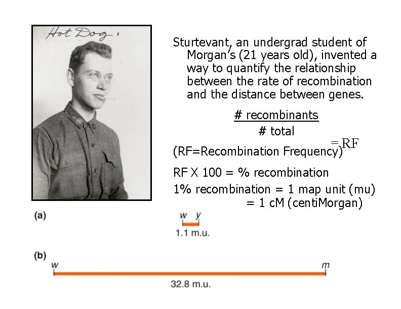
Sturtevant, an undergrad student of Morgan’s (21 years old), invented a way to quantify the relationship between the rate of recombination and the distance between genes. # recombinants # total = RF (RF=Recombination Frequency) RF X 100 = % recombination 1% recombination = 1 map unit (mu) = 1 c. M (centi. Morgan)

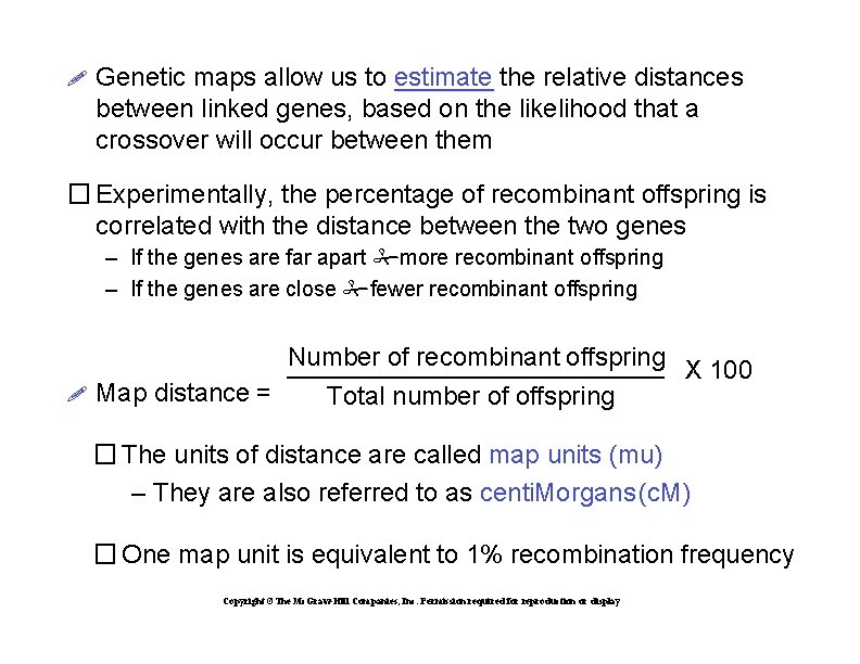
Genetic maps allow us to estimate the relative distances between linked genes, based on the likelihood that a crossover will occur between them � Experimentally, the percentage of recombinant offspring is correlated with the distance between the two genes – If the genes are far apart more recombinant offspring – If the genes are close fewer recombinant offspring Number of recombinant offspring X 100 Map distance = Total number of offspring � The units of distance are called map units (mu) – They are also referred to as centi. Morgans (c. M) � One map unit is equivalent to 1% recombination frequency Copyright ©The Mc. Graw-Hill Companies, Inc. Permission required for reproduction or display

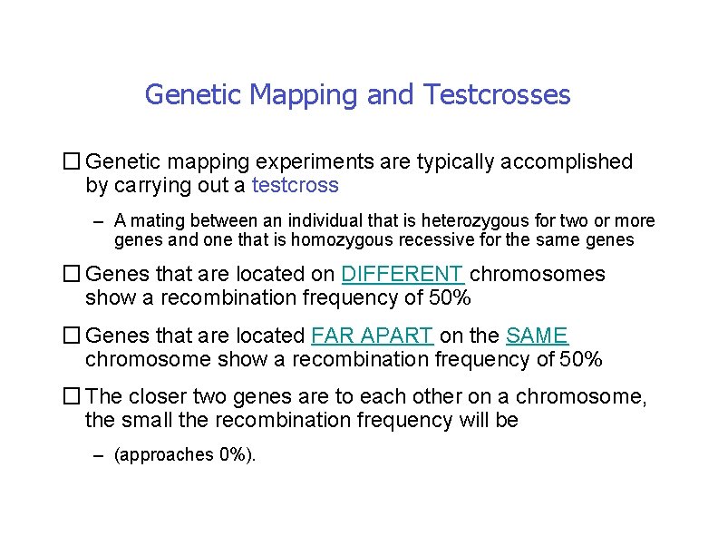
Genetic Mapping and Testcrosses � Genetic mapping experiments are typically accomplished by carrying out a testcross – A mating between an individual that is heterozygous for two or more genes and one that is homozygous recessive for the same genes � Genes that are located on DIFFERENT chromosomes show a recombination frequency of 50% � Genes that are located FAR APART on the SAME chromosome show a recombination frequency of 50% � The closer two genes are to each other on a chromosome, the small the recombination frequency will be – (approaches 0%).

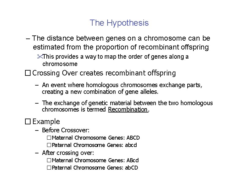
The Hypothesis – The distance between genes on a chromosome can be estimated from the proportion of recombinant offspring This provides a way to map the order of genes along a chromosome � Crossing Over creates recombinant offspring – An event where homologous chromosomes exchange parts, creating a new combination of gene alleles. – The exchange of genetic material between the two homologous chromosomes is termed Recombination. � Example – Before Crossover: �Maternal Chromosome Genes: ABCD �Paternal Chromosome Genes: abcd – After crossing over: �Maternal Chromosome Genes: ABcd �Paternal Genes: ab. CD Copyright. Chromosome ©The Mc. Graw-Hill Companies, Inc. Permission required for reproduction or display

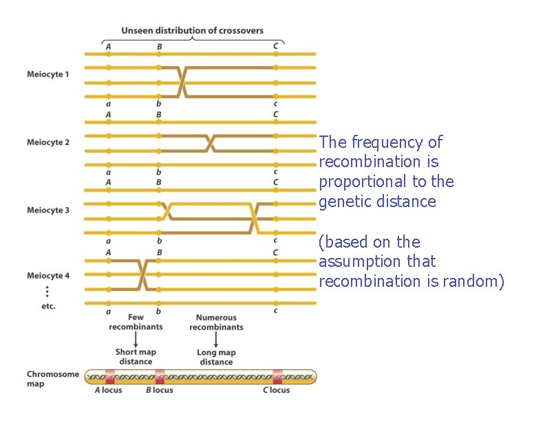
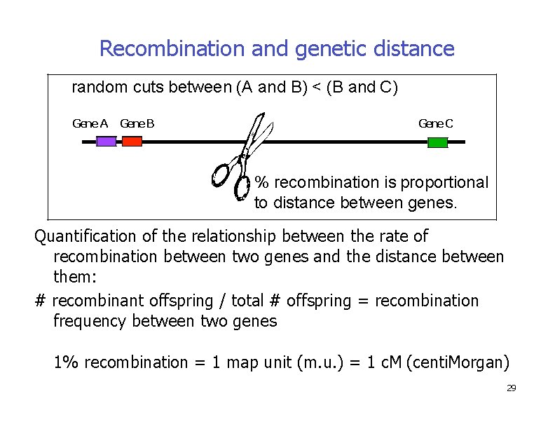
The frequency of recombination is proportional to the genetic distance (based on the assumption that recombination is random)

Recombination and genetic distance random cuts between (A and B) < (B and C) Gene A Gene B Gene C % recombination is proportional to distance between genes. Quantification of the relationship between the rate of recombination between two genes and the distance between them: # recombinant offspring / total # offspring = recombination frequency between two genes 1% recombination = 1 map unit (m. u. ) = 1 c. M (centi. Morgan) 29

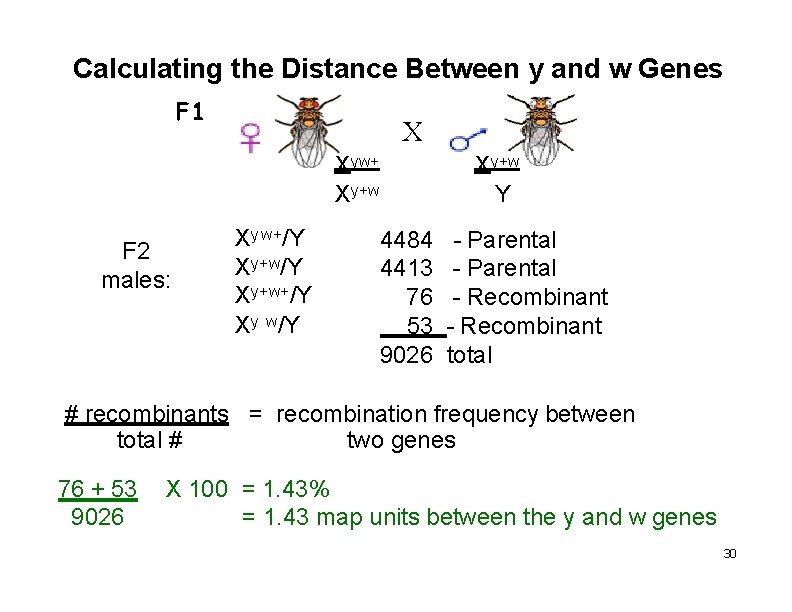
Calculating the Distance Between y and w Genes F 1 X Xyw+ Xy+w F 2 males: Xy w+/Y Xy+w+/Y Xy w/Y 4484 4413 76 53 9026 Xy+w Y - Parental - Recombinant total # recombinants = recombination frequency between total # two genes 76 + 53 9026 X 100 = 1. 43% = 1. 43 map units between the y and w genes 30

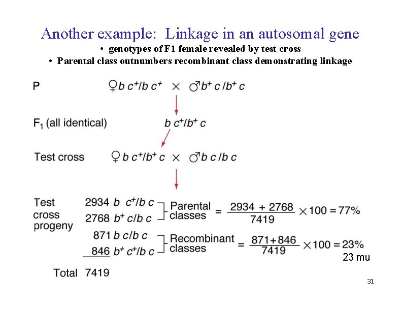
Another example: Linkage in an autosomal gene • genotypes of F 1 female revealed by test cross • Parental class outnumbers recombinant class demonstrating linkage 23 mu 31

Summary of linkage and recombination “rules” � Genes close together on the same chromosome are linked and do not segregate independently � Linked genes lead to a larger number of parental class than expected in double heterozygotes � Mechanism of recombination is crossing over � Chiasmata are the visible signs of crossing over � Farther away genes are, the greater the opportunity for chiasmata to form � Recombination frequencies reflect physical distance between genes � Recombination frequencies between two genes vary from 0% to 50% 32

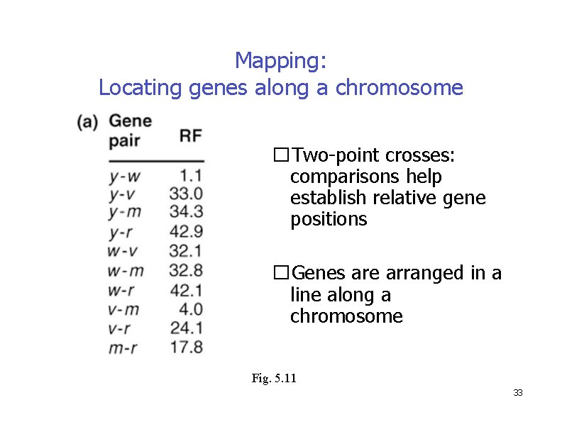
Mapping: Locating genes along a chromosome �Two-point crosses: comparisons help establish relative gene positions �Genes are arranged in a line along a chromosome Fig. 5. 11 33

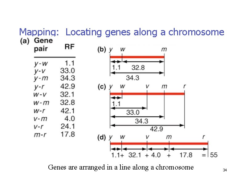
Mapping: Locating genes along a chromosome Fig. 5. 11 Genes are arranged in a line along a chromosome 34

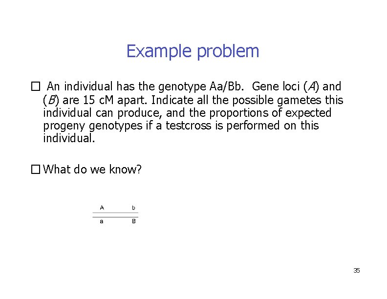
Example problem � An individual has the genotype Aa/Bb. Gene loci (A) and (B) are 15 c. M apart. Indicate all the possible gametes this individual can produce, and the proportions of expected progeny genotypes if a testcross is performed on this individual. � What do we know? 35

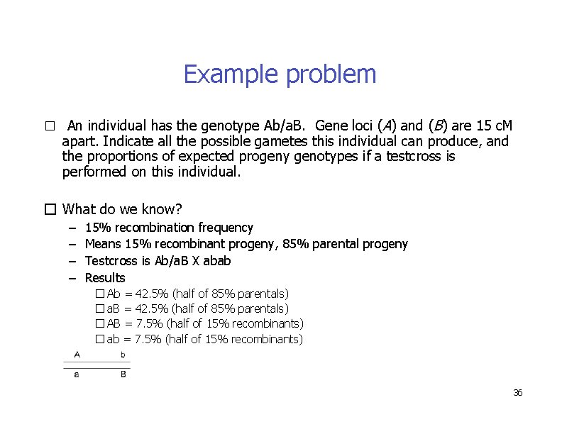
Example problem � An individual has the genotype Ab/a. B. Gene loci (A) and (B) are 15 c. M apart. Indicate all the possible gametes this individual can produce, and the proportions of expected progeny genotypes if a testcross is performed on this individual. � What do we know? – – 15% recombination frequency Means 15% recombinant progeny, 85% parental progeny Testcross is Ab/a. B X abab Results � Ab = 42. 5% (half of 85% parentals) � a. B = 42. 5% (half of 85% parentals) � AB = 7. 5% (half of 15% recombinants) � ab = 7. 5% (half of 15% recombinants) 36

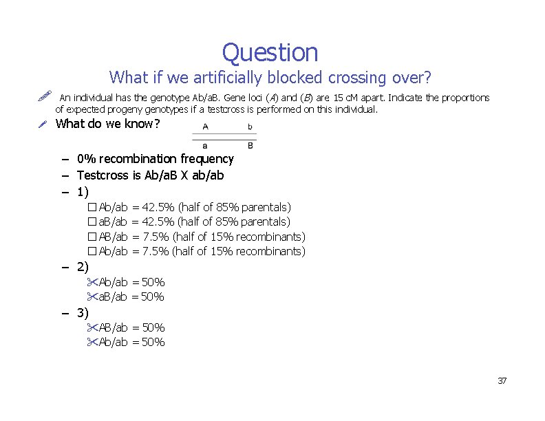
Question What if we artificially blocked crossing over? An individual has the genotype Ab/a. B. Gene loci (A) and (B) are 15 c. M apart. Indicate the proportions of expected progeny genotypes if a testcross is performed on this individual. What do we know? – 0% recombination frequency – Testcross is Ab/a. B X ab/ab – 1) � Ab/ab = 42. 5% (half of 85% parentals) � a. B/ab = 42. 5% (half of 85% parentals) � AB/ab = 7. 5% (half of 15% recombinants) � Ab/ab = 7. 5% (half of 15% recombinants) – 2) Ab/ab = 50% a. B/ab = 50% – 3) AB/ab = 50% Ab/ab = 50% 37

Limitations of two point crosses �Difficult to determine gene order if two genes are close together �Actual distances between genes do not always add up �Pairwise crosses are time and labor consuming 38