Linkage Chromosome mapping by recombination Meiosis is the

Linkage Chromosome mapping by recombination Meiosis is the basis of transmission genetics The recombination that occurs during meiosis (in heterozygotes) generates data that are a useful tool for making linkage maps Linkage maps assist in understanding evolution, synteny, and selection response

Populations for Linkage Analysis Parent 1 F 1 Parent 2

Doubled Haploids Parent 1 Parent 2 F 1 Gametes

What is Linkage? P 2 P 1 Two loci: -Spike color - Plant height Linked 14 parental: 2 nonparental Independent 8 parental: 8 nonparental ×

Linkage • The association of two or more phenotypic characters in inheritance because the genes controlling these characters are located in the same chromosome. • The closer the gene locations, the stronger the association • Genes carried by the same chromosome are members of the same linkage group • The number of linkage groups corresponds, therefore, to the basic number of chromosomes in the organism in question.

Chromosomes Plant 2 n = _X = _ Genes Arabidposis thaliana 2 n = 2 x = 10 27, 000 Fragaria vesca 2 n = 2 x = 14 35, 000 Theobroma cacao 2 n = 2 x = 20 29, 000 Zea mays 2 n = 2 x = 20 40, 000

Linkage • Crossing over refers to the physical exchange between homologous chromosomes. Meiotic crossing over is a potent source of genetic variability. • Recombination is the genetic result of crossing over and is detected by new combinations of alleles at two or more loci.

Meiosis Prophase I (5 stages) 1. Leptonema: Longitudinal duality of chromosomes not discernible. 2. Zygonema: Pairing of homologous chromosomes. Formation of synaptonemal complex and zygotene DNA synthesis. 3. Pachynema: Pairing persists: synaptonemal complex + crossovers. Bivalent = 2 homologous chromosomes = 2 sets of 2 chromatids. Crossing over occurs (chiasma; chiasmata). 4. Diplonema: Synaptonemal complex dissolves; visualize longitudinal duality. 5. Diakinesis: Continued bivalent contraction.

Crossing Over www. accessexcellence. org

Linkage Complete: Pairs of loci are so close together that crossing over rarely occurs and recombinant types are generally not recovered. 1, 2, 3……. . 100 0 10 0 crossovers between loci 1, 2, 3 and 10 crossovers between the cluster of loci 1/2/3 and locus 100 (in a population of 100 individuals) Partial: Pairs of loci are sufficiently far apart that some recombinant types are recovered. The "distance" between genes ranges from a few percent recombination to 50% recombination.

Linkage Terms describing the allelic condition at linked loci cis aka coupling A……. . B a……. . b trans aka repulsion A……. . b a……. . B

Linkage At Pachynema, there can be breakage of chromatids, followed by their fusion with sister chromatids, or with nonsister chromatids. As long as orientation corresponds, reciprocal exchanges between sister chromatids will not be detected and will not lead to genetic variability.

Linkage Keys points in non-sister chromatid exchange: • Crossing over does not involve loss or addition of chromatin • Only two chromatids are involved in any single crossover event • There may be multiple crossovers between non-sister chromatids • Any combination of crossover configurations can occur, and the outcome of such configurations can be radically different

Linkage Factors affecting meiotic crossing over Sex chromosomes

Linkage Dioecy Evolution of sex chromosomes from autosomes • Accumulation of sex-determining genes on a single chromosome with no homolog prevents recombination between sex-determining genes

Linkage Factors affecting meiotic crossing over Position on chromosome

Linkage Types of Crossovers Single crossover 2 -strand double crossover 3 -strand double crossover 4 -strand double crossover

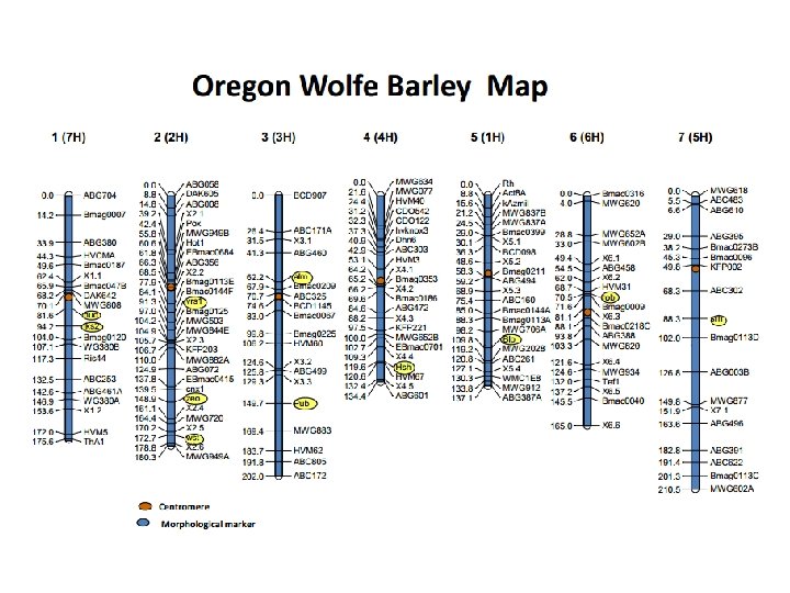
Oregon Wolfe Barley Map 187 classical loci

Linkage Relationships Oregon Wolfe Barley Parents OWB Dominant 2 -row; normal starch; hulled grain; long awns VV WW NN LL V W N L OWB Recessive 6 -row; waxy starch; naked grain; short awns vv ww nn ll v w n l Locus abbreviations and alleles Vrs 1 = V: V, v GBSS = W: W, w Nud = N: N, n LKs 2 = L: L, l

An example of how independent assortment and recombination could lead to an entirely new combination of traits: 2 -row; waxy starch; hulled grain; short awn OWB Dominant 2 -row; normal starch; hulled grain; long awns VV WW NN LL V V v v x W NL w nl OWB Recessive 6 -row; waxy starch; naked grain; short awns vv ww nn ll V v F 1 W NL w nl

Meiosis 1 & Crossing Over – Cell 1 Ch 2 v V v v V V v After Pre-meiotic Heterozygous parent DNA replication v V V v Pairing and crossing over v V V Anaphase I w W w w W W n l N L n l Ch 7 N L N L

Meiosis 2 & Crossing Over – Cell 1 Anaphase II V Ch 2 v NL W Ch 7 V w Ch 2 n l W Ch 7 v w 2 row, non-waxy, hulled, long awn V W NL 6 row, waxy, hulled, long awn 2 row, non-waxy, naked, short awn v w NL V W n l 6 row, waxy, naked, short awn v Ch 2 w n l Ch 7 NL n l Non-Recombinant Non-Recombinant

Meiosis 1 & Crossing Over – Cell 2 Ch 2 V v V V v v V After Pre-meiotic Heterozygous parent DNA replication V v v V Pairing and crossing over V v v Anaphase I w W w w W W n l N L n l Ch 7 N L N L

Meiosis 2 & Crossing Over – Cell 2 Anaphase II V w Ch 2 Ch 7 V Ch 2 Ch 7 v N L w n l W v n l W 2 row, waxy, naked, short awn V w n l 6 row, non-waxy, naked, short awn 2 row, waxy, hulled, short awn v W n l Recombinant V w N L Recombinant v W N L 6 row, non-waxy, hulled, long awn Ch 2 Ch 7 N L Non-Recombinant

Doubled Haploid Phenotypes 2 row, non-waxy, hulled, long awn 6 row, waxy, hulled, long awn 2 row, non-waxy, naked, short awn 6 row, waxy, naked, short awn 2 row, waxy, naked, short awn 6 row, non-waxy, naked, short awn 2 row, waxy, hulled, short awn 6 row, non-waxy, hulled, long awn Ch 2 V W NL V v W w NL NL v V w W NL n l V v W w n l n v w l n l V w n l V v w W n l v V W w n l N L Recombinant V v w W N L Non-Recombinant v W N L Ch 7 Non-Recombinant Non-Recombinant

Dihybrid Ratio for Doubled Haploids (2/4 loci) Gametes VW Vw v. W vw DH VVWW VVww vv. WW vvww Class Non. Recombinant recombinant Recombinant 1 1 0. 25 Note: The “recombinant “ types in this case (between the V and W loci) are not due to crossovers. They are due to random alignment of paired homologous chromosomes at Metaphase I

Linkage Test – 2/6 row v waxy/non Gametes VW Vw v. W vw DH VVWW VVww vv. WW vvww Non. Recombinant recombinant Recombinant 0. 25 Expected 20. 5 Observed 20 15 25 22 (O-E)2/E 0. 012 1. 476 0. 988 0. 110 = 2. 586; P=0. 460; Null hypothesis of no linkage accepted Independent Assortment : Loci are on different chromosomes Random alignment of chromosomes at Metaphase 1 (slide 22 vs. slide 24) 2 [3]

Linkage Test – waxy/non v hulled/naked Gametes WN Wn w. N Wn DH WWNN WWnn ww. NN wwnn Non. Recombinant recombinant Recombinant 0. 25 Expected 20. 5 Observed 27 18 13 24 (O-E)2/E 2. 061 0. 305 2. 744 0. 598 = 5. 707; P=0. 128; Null hypothesis of no linkage accepted Independent Assortment: Sufficient crossovers between loci far enough apart on same chromosome 2 [3]

Linkage Test – waxy/non v long/short awn Gametes WL Wl w. L wl DH WWLL WWll ww. LL wwll Non. Recombinant recombinant Recombinant 0. 25 Expected 20. 5 Observed 26 19 20 17 (O-E)2/E 1. 476 0. 110 0. 012 0. 598 = 2. 195; P=0. 533; Null hypothesis of no linkage accepted Independent Assortment: Sufficient crossovers between loci far enough apart on same chromosome 2 [3]

Link Test – naked/hulled v long/short awn Gametes NL Nl n. L nl DH NNLL NNll nn. LL nnll Non. Recombinant recombinant Recombinant 0. 25 Expected 20. 5 Observed 37 3 9 33 (O-E)2/E 13. 280 14. 939 6. 451 7. 622 = 42. 293; P=<0. 001; Null hypothesis of no linkage rejected Not Independent Assortment = linkage Few crossovers between loci close together on same chromosome 2 [3]

Recombination Parent 1 2 Gametes 3 4 1 2 A B a b 3 4 A B A b a B a b Non Recombinant n 1 Recombinant n 2 Recombinant n 3 Non Recombinant n 4 Total Recombination frequency N

Recombination Frequency Parentals (Non-recombinants) >> Recombinants = linkage Linkage is calculated as the total Recombinant types/ total population size Nl (n 2) = 3; n. L (n 3) = 9; N = 82 r = (n 2+n 3)/N; r= 12/82 = 14. 6% • N and L are approximately 14. 6 map units apart • They are linked “The association of two or more phenotypic characters in inheritance because the genes controlling these characters are located in the same chromosome”

Three Point Linkage Test r. WN=0. 39 r. NL=0. 14 N W L r. WL=0. 48 The recombination frequency over the interval W – L (r. WL) is greater than either r. WN or r. NL therefore W and L are the two loci furthest apart and N is likely to lie between them. N is likely to be closer to L as r. WN > r. NL.

Recombination and Map Distance • % recombination values are biased due to double crossovers • Double crossovers can give parental combinations of alleles and therefore underestimate the % recombination at values of ~ 10% recombination and higher • At values of ~ 10% recombination and less, double crossovers occur less often than expected • % recombination values are not additive: the maximum of recombination is 50% Therefore the centi. Morgan – a computed value derived from the observed % recombination

Non-Additivity of recombination frequencies r. BC r. AB A C B r. AC The recombination frequency over the interval A – C (r. AC) is less than the sum of r. AB and r. BC : r. AC < r. AB + r. BC. This is because (rare) double recombination events (a recombination in both A - B and B - C) do not contribute to recombination between A and C.

Map Distance Measures Distance (c. M) Haldane =-0. 5*LN(1 -2*r) Distance (c. M) Kosambi=0. 25*LN((1+2*r)/(1 -2*r)) The centi. Morgan is a unit of distance without a physical basis. This is readily apparent in organisms with large genomes, where the ratio of c. M to base pairs can vary enormously across the genome

Mapping Function & Recombination Mapping Functions

Oregon Wolfe Barley Map 187 classical loci 1 H 0 7 12 17 22 25 28 30 36 49 59 64 79 109 119 126 150 151 152 160 162 166 2 H 0 BCD 1434 1 Ds. T-66 13 41 Act 8 A 45 Rbg. MD MWG 837 B 47 scind 00046 50 ABC 165 C 62 Bmac 0399 68 GBM 1007 69 BCD 098 GBM 1042 72 Bmag 0211 75 BG 369940 77 ABC 160 90 96 102 105 JS 10 C 110 MWG 706 A 111 KFP 170 112 115 MWG 2028133 ABC 261 150 KFP 257 B 152 WMC 1 E 8 161 MWG 912 173 ABG 387 A scssr 04163176 179 185 193 3 H ABG 058 scind 02622 0 ABG 008 scssr 10226 69 scssr 07759 12 GBM 1066 Pox scssr 03381 37 41 Hot 1 Ebmac 0684 45 scssr 02236 48 scssr 00334 63 ABG 356 65 GBM 1023 73 scsnp 03343 vrs 1 Bmag 0125 98 Ds. T-41 MWG 503 GBM 1062 123 KFP 203 MWG 882 A ABG 072 Ebmc 0415 147 cnx 1 160 Zeo 1 GBM 1019 165 Aglu 4 183 MWG 720 191 GBM 1012 MWG 949 A 202 scssr 08447 4 H 0 20 23 29 GBM 1074 30 MWG 798 B 31 35 Dst-27 BCD 706 41 44 alm Bmac 0209 ABC 325 50 Ds. T-67 scssr 25691 52 ABG 377 Bmag 0225 60 61 68 80 ABG 499 81 84 93 scsnp 00940 95 96 102 113 ABG 004 114 scind 02281117 MWG 883 127 HVM 62 ABC 805 ABC 172 5 H MWG 634 MWG 077 HVM 40 CDO 542 scsnp 01648 0 CDO 122 7 hvknox 3 12 ABC 303 13 scssr 20569 CDO 795 DST-46 41 scind 03751 48 scind 04312 a 61 Tef 2 scind 01728 62 GBM 1020 63 Bmag 0353 scind 10455 91 scssr 14079 94 ABG 472 96 GBM 1059 100 KFP 221 111 Ebmac 0701 MWG 652 B GBM 1048 135 Hsh 142 HVM 67 148 KFP 241. 1 153 ABG 601 184 188 203 224 228 229 236 239 253 255 6 H scssr 02306 MWG 618 0 ABC 483 ABG 610 36 ABG 395 48 scssr 02503 55 NRG 045 A 67 scsnp 04260 70 73 Ale 75 76 ABC 302 scind 16991 87 scssr 15334 97 scsnp 06144103 107 srh 134 RSB 001 A 142 scsnp 00177145 0 SU-STS 1 153 ABG 003 B 157 170 171 173 Tef 3 MWG 877 ABG 496 E 10757 A scsnp 02109 ABG 391 JS 10 B ABC 622 Ds. T-33 MWG 602 A scssr 03906 7 H Bmac 0316 0 16 24 MWG 602 B 31 JS 10 A 33 GBM 1021 GBM 1068 BG 299297 72 HVM 31 73 rob 74 scssr 02093 87 Bmag 0009 91 ABG 474 94 ABG 388 scsnp 21226 103 MWG 820 104 108 GBM 1008 124 scind 04312 b 128 GBM 1022 136 Bmac 0040 137 Ds. T-32 B 138 Ds. T-28 149 Ds. T-74 151 MWG 798 A 169 MWG 514 179 184 191 215 218 ABG 704 GBSS-I AW 982580 CDO 475 MWG 089 ABG 380 scsnp 00460 ABC 255 ABC 165 D scssr 15864 GBM 1030 MWG 808 DAK 642 scsnp 00703 MWG 2031 nud lks 2 ABC 1024 Bmag 0120 Ds. T-30 WG 380 B ABC 310 B Ris 44 ABC 253 ABG 461 A WG 380 A Ds. T-69 GBM 1065 KFP 255 Th. A 1 124 – 108 = 16 c. M on this map vs. 14% two-locus recombination

Oregon Wolfe Barley Map 187 classical + 555 pilot-OPA 1 + 467 pilot-OPA 2 = 1209 loci 111 - 96 = 15 c. M on this map vs. 14% two-locus recombination

Recombination vs. Map Distance 94. 2 – 81. 6 = 12. 6 c. M on this map vs. 14% two-locus recombination c. M < % recombination? ? ?

Value of Genetic Linkage Maps • Determine order of loci in the chromosome • Determine how likely it is that non-parental combinations of alleles at linked loci will be obtained • Determine if trait relationships are due to linkage or pleiotropy • Create complete linkage maps (average ~ 100 c. M/chromosome) where # chromosomes (n level) = number of linkage groups • Build a platform for cloning genes • A framework for whole genome sequences • Identify genes controlling quantitative traits

Graphical Genotypes Visualise the consequences of recombination Graphical genotypes (haplotypes) of selected a mapping population

Making Linkage Maps • Linkage analysis is now an "automated" procedure Ø Data on thousands, tens of thousands of loci • Key issues in linkage map construction are locus order and distance • The likelihood odds (LOD) score is a test statistic that is used to test the hypothesis that there is no linkage Ø LOD of 3. 00 is approximately equal to P ~. 001 Ø LOD > 3 then one concludes that two loci are indeed linked.

Locus ordering Number of orders among k loci Number of triplets among k loci No. of loci k Possible orders No. of triplets 2 1 0 3 3 1 5 60 10 10 1, 814, 400 120 20 1. 22 X 1018 1, 140 40 4. 08 X 1047 9, 880

Oregon Wolfe Barley Map 187 classical loci

Oregon Wolfe Barley Map 187 classical + 722 DAr. T = 909 loci

Oregon Wolfe Barley Map 187 classical + 555 pilot-OPA 1 + 467 pilot-OPA 2 = 1209 loci

Oregon Wolfe Barley Map 187 classical + 555 pilot-OPA 1 + 467 pilot-OPA 2 + 722 DAr. T = 1931 loci

Oregon Wolfe Barley Linkage Map - (2383 loci, Haldane c. M)

Oregon Wolfe Barley Linkage Map (2383 loci + 463 RAD = 2846 loci)

Map Relationships Homoeology: Chromosomes, or chromosome segments, which are similar in terms of the order and function of the genetic loci. Homoeologous chromosomes may occur within a single allopolyploid individual (e. g. the A, B, and D genomes in wheat) Or they may be found in related species (e. g. the 1 A, 1 B, 1 D series in wheat and the 1 H of barley)

Genome Organisation & Maps Synteny or syntenic regions: Genetic loci that are linked on the same chromosome Chromosomes and/or sections of chromosomes are reassembled in different configurations in related organisms Fragaria: Prunus

Genome Organisation & Maps Orthology: Genes in different species which are so similar in sequence that they are assumed to have originated from a single ancestral gene. doi/10. 1371/journal. pcbi. 1000703

Interference and Mapping

Interference • Interference means that recombination events in adjacent intervals interfere. The occurrence of an event in a given interval may reduce or enhance the occurrence of an event in its neighbourhood. • Positive interference refers to the ‘suppression’ of recombination events in the neighbourhood of a given one. • Negative interference refers to the opposite: enhancement of clusters of recombination events. • Positive interference results in less double recombinants (over adjacent intervals) than expected on the basis of independence of recombination events. r. AC=r. AB+r. BC-2 Cr. ABr. BC

Interference A B C a b c Coefficient of coincidence C = coefficient of coincidence For N individuals, the expected number of double crossovers = r. ABr. BCN Interference I = 1 - C

Coefficient of Coincidence (C) Observed 22 24 16 14 8 10 2 4

Interference • No interference – C = 1 and Interference = 1 -C = 0 • Complete interference – C = 0 and Interference = 1 -C = 1 • Negative interference – C > 1 and Interference = 1 -C < 0 • Positive interference – C < 1 and Interference = 1 -C > 0