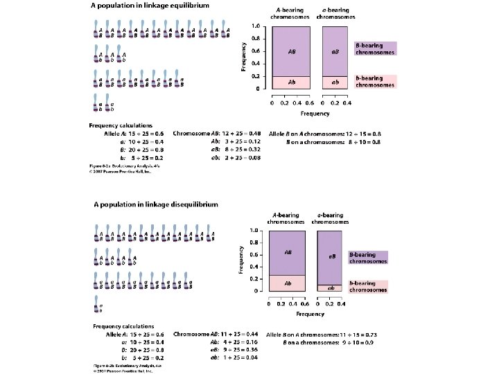
Linkage and Linkage Disequilibrium AB 25 A B

Linkage and Linkage Disequilibrium AB = 25% A B Ab = 25% a. B = 25% a b ab = 25% A B a b AB = 50% Ab = 0% a. B = 0% ab = 50% f(Ab) = f(A) x f(b) B b A a f(Ab) ≠ f(A) x f(b) B b A a A locus and B locus are in Linkage Disequilibrium D = f(AB) x f(ab) - f(Ab) x f(a. B) Maximum with no recombination D = 0 with free recombination (linkage equilibrium)

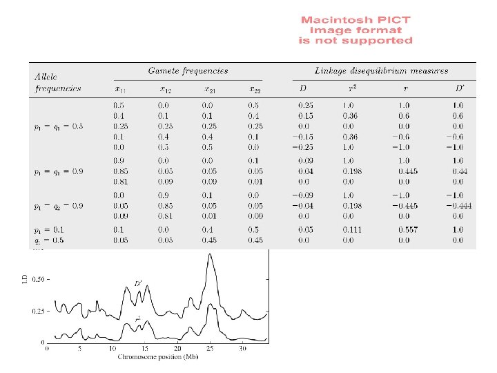
Linkage equilibrium: Are alleles at separate loci paired at random? D = x 11 − p 1 q 1 D = x 22 − p 2 q 2
 x f(ab)")
A locus and B locus are in Linkage Disequilibrium D = f(AB) x f(ab) - f(Ab) x f(a. B) Maximum with no recombination D -> 0 with free recombination (linkage equilibrium) When allele frequencies are intermediate: f(A) = f(a) = f(B) = f(b) = 0. 5, and maximal LD occurs so that no recombinants are present: f(AB) = f(ab) = 0. 5, so D = 0. 5 x 0. 5 – 0. 0 x 0. 0 = 0. 25 When allele frequencies are skewed: f(A) = 0. 9, f(a) = 0. 1; f(B) = 0. 9, f(b) = 0. 1 and maximal LD occurs so that no recombinants are present, D is less than 0. 25: f(AB) = 0. 9, and f(ab) = 0. 1, so D = 0. 9 x 0. 1 – 0. 0 x 0. 0 = 0. 09

LD as a two-locus Hardy Weinberg problem
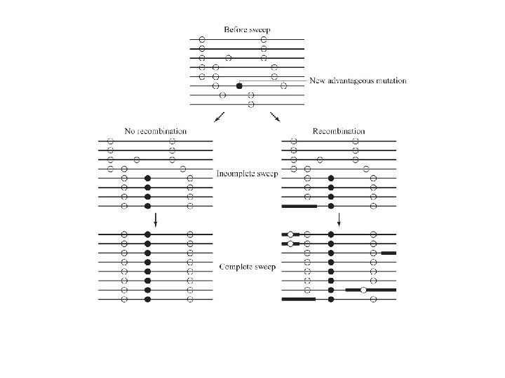
 decays with distance and time A B a b r= Rate")
Linkage disequilibrium (LD) decays with distance and time A B a b r= Rate of recombination AB = (1 -r)/2 Ab = r/2 a. B = r/2 ab = (1 -r)/2

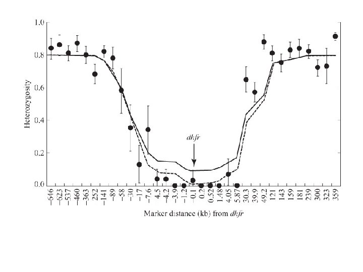
Empirical demonstration of the Decay of LD over time

Epistasis
 M. lewisii F 2’s F 1")
QTL for flower traits in Mimulus (monkey flowers) M. lewisii F 2’s F 1 M. cardinalis Different pollinators

Genetic map of monkey flower http: //www. genetics. org/cgi/content/full/159/4/1701/F 1
mapping: Screen for marker-trait associations in F 2 s or RILs")
Quantitative trait locus (QTL)mapping: Screen for marker-trait associations in F 2 s or RILs Parentals F 1 M, Q M, Q F 2 Inbreed to make Recombinant inbred lines (RILs) Scan genome for association Between molecular marker and phenotype Association between Molecular marker (M) and QTL(Q) Small m, q M, Q Large

QTL here Marker here http: //isotope. bti. cornell. edu/img/intro/qtl_fig_2. gif QTL Mapping: detecting an association between a genetic marker (M) and a gene affecting a quantitative trait (Q). QTL mapping works because there is linkage disequilibrium (LD) between the marker (M) and the QTL (Q): mm marker genotypes are correlated with small size MM marker genotypes are correlated with large size

Most traits in organisms Show continuous variation How do we find the genes That affect these “quantitative” traits Scan the genome for Nucleotide sites that Co-vary with the phenotype

Genome wide association studies: GWAS Mutation “causing” variation in height Tall Short A A G G Adjacent SNPs are linked Distant sites show no genotype-phenotype association Problem: how do we find the causal SNPs? Needle in a haystack

What is better: More recombination, more markers? Parentals F 1 M, Q M, Q F 2 Inbreed to make Recombinant inbred lines (RILs) Scan genome for association Between molecular marker and phenotype Association between Molecular marker (M) and QTL(Q) Small m, q M, Q Large

How does DNA evolve? 1 ATGCCCCAACTAAATACTACCGTATGGCCCACCATAATTACCCCCATACT 50 Human ||||||||||||||| Chimp 1 atgccccaactaaataccgccgtatgacccaccataattacccccatact 50. . . 51 CCTTACACTATTCCTCATCACCCAACTAAAAATATTAAACACAAACTACC 100 ||| ||||||||||||||| 51 cctgacactatttctcgtcacccaactaaaaatattaaattcaaattacc 100. . . 101 ACCTCCCTCACCAAAGCCCATAAAAAATTATAACAAACCC 150 | ||||||||||| || || |||||| 101 atctacccccctcaccaaaacccataaaaaactacaataaaccc 150. . . 151 TGAGAACCAAAATGAACGAAAATCTGTTCGCTTCATTGCCCCCACA 200 ||||||||||||| ||||| 151 tgagaaccaaaatgaacgaaaatctattcgcttcattcgctgcccccaca 200 201 ATCC 204 |||| 201 atcc 204

Measuring DNA Evolution • • • Align sequences between species Determine length of sequences, L Count number of differences Divergence = proportion of differences D = p-distance = (number of differences) / (length of sequence) Rate of divergence = (sequence divergence) / (age of common ancestor) = D / time Rate of substitution = D / 2 x time Example: 5 differences in 100 D = 0. 05, t = 6 million years Divergence = 0. 05/6 x 106 Divergence = 8. 3 x 10 -9
 = ¼ + ¾")
Jukes Cantor One parameter model = rate of substitution PA(t) = ¼ + ¾ e-4 t = probability that A remains A at time t PNN = ¼ + ¾ e-8 t = probability that two sequences have the same nucleotide at N D = proportion of different nucleotides = 1 - PNN Dhat = 3/4(1 -e-8 t) K = - ¾ ln (1 -4/3 p) where p = proportion of nucleotide differences (# diffs. /total bp)

Kimura two-parameter model = rate of transition substitution b b b = rate of transversion substitution PAA(t) = ¼ + ¾ e-4 bt + ½ e-2( +b)t = probability that A remains A at time t K = ½ ln(1/[1 - 2 P-Q]) + ¼ ln(1/[1 -2 Q]) where P = proportion of transitional differences Q = proportion of transversional differences
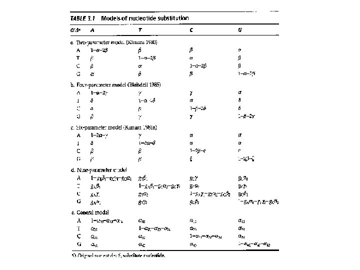

Comparison of models • • P-distance Jukes Cantor Kimura 2 -parameter Tamura-Nei • Etc…

Molecular clocks Approximately constant Divergence of proteins K = • f 0 Rate of substitution = Mutation rate x proportion of neutral mutations “Saturation” due to multiple Hits in DNA evolution
 nodes Taxa = Taxon 1 OTUs =")
Anatomy of a phylogenetic tree Terminal (external) nodes Taxa = Taxon 1 OTUs = Operational taxonomic units External branch Internal branch Taxon 2 Taxon 3 Taxon 4 Taxon 5 Taxon 6 Polytomy Non-dichotomous splitting Internal nodes Root

Relative rate test • KAC = KBC • KOC is shared • Tajima test • (m 1 -m 2)2 / (m 1+m 2) • Chi square, df=1 Species O m 1 m 2 Species A Species B Species C
 substitution rate")
DNA test of neutrality • • • Neutral prediction: amino acid (nonsynonymous) substitution rate (d. N) should be lower than silent (synonymous) substitution rate (d. S) True for most genes – • Follows from functional constraint argument Different for Major Histocompatibility Complec (MHC) loci – • Antigen binding sites: d. N/d. S > 1 “positive” selection Antigen recognition sequence shows d. N > d. S Rest of molecule shows d. N > d. S, as expected Amino acid mutations are favored in antigen recognition region Promotes diversity, better recognition of foreign peptides http: //depts. washington. edu/rhwlab/dq/3 structure. html Rest of molecule: d. N/d. S < 1 Negative (purifying) selection

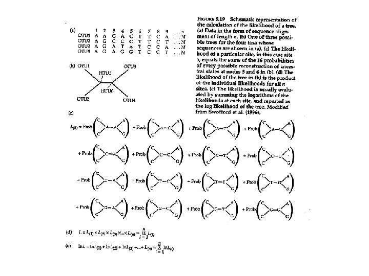
Maximum likelihood • Likelihood of observing the data set – Assuming a given tree – Assuming a given model of DNA evolution • L = P(data|tree) • Consider 4 -taxon cases within a tree OTU 1 HTU 1 OTU 1 – For each site, Identify nucleotides at each of the four taxa – Assume all 16 pairs of nucleotides at internal nodes – Likelihood of observed 4 terminal nucleotides = sum of 16 independent probabilities – Repeat likelihoods for each position in alignment – Likelihood of tree = product of individual likelihoods OTU 1 HTU 1 OTU 1 • L = P Li for i = 1 to n positions in alignment (or sum of log likelihoods) • Calculate likelihood for other trees; choose tree with maximum likelihood
- Slides: 34