Linkage analysis basic principles Manuel Ferreira Pak Sham

Linkage analysis: basic principles Manuel Ferreira & Pak Sham Boulder Advanced Course 2005

Outline 1. Aim 2. The Human Genome 3. Principles of Linkage Analysis 4. Parametric Linkage Analysis 5. Nonparametric Linkage Analysis

1. Aim

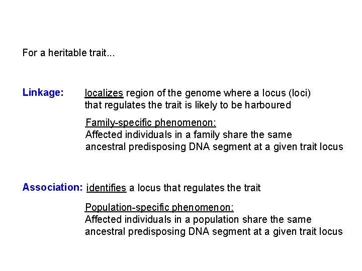
For a heritable trait. . . Linkage: localizes region of the genome where a locus (loci) that regulates the trait is likely to be harboured Family-specific phenomenon: Affected individuals in a family share the same ancestral predisposing DNA segment at a given trait locus Association: identifies a locus that regulates the trait Population-specific phenomenon: Affected individuals in a population share the same ancestral predisposing DNA segment at a given trait locus

2. Human Genome

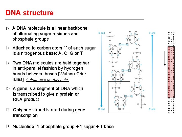
DNA structure A DNA molecule is a linear backbone of alternating sugar residues and phosphate groups Attached to carbon atom 1’ of each sugar is a nitrogenous base: A, C, G or T Two DNA molecules are held together in anti-parallel fashion by hydrogen bonds between bases [Watson-Crick rules] Antiparallel double helix A gene is a segment of DNA which is transcribed to give a protein or RNA product Only one strand is read during gene transcription Nucleotide: 1 phosphate group + 1 sugar + 1 base

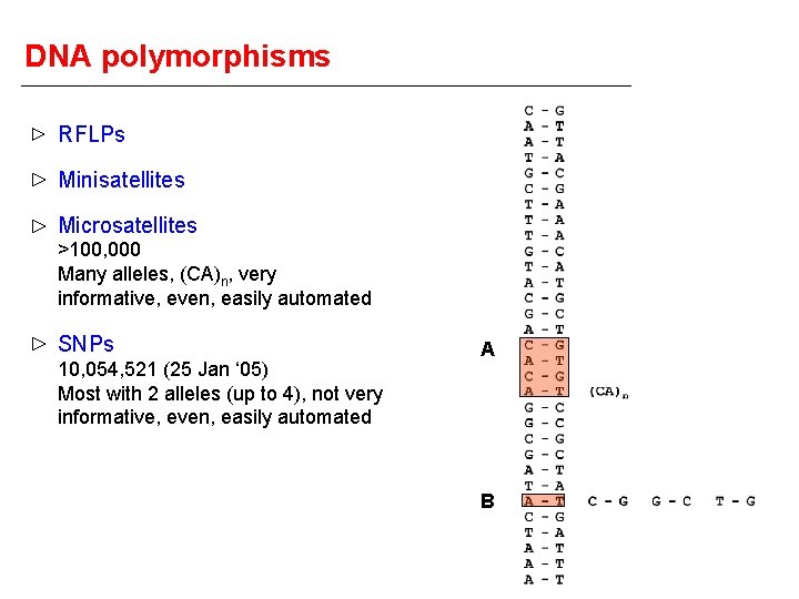
DNA polymorphisms RFLPs Minisatellites Microsatellites >100, 000 Many alleles, (CA)n, very informative, even, easily automated SNPs 10, 054, 521 (25 Jan ‘ 05) Most with 2 alleles (up to 4), not very informative, even, easily automated A B

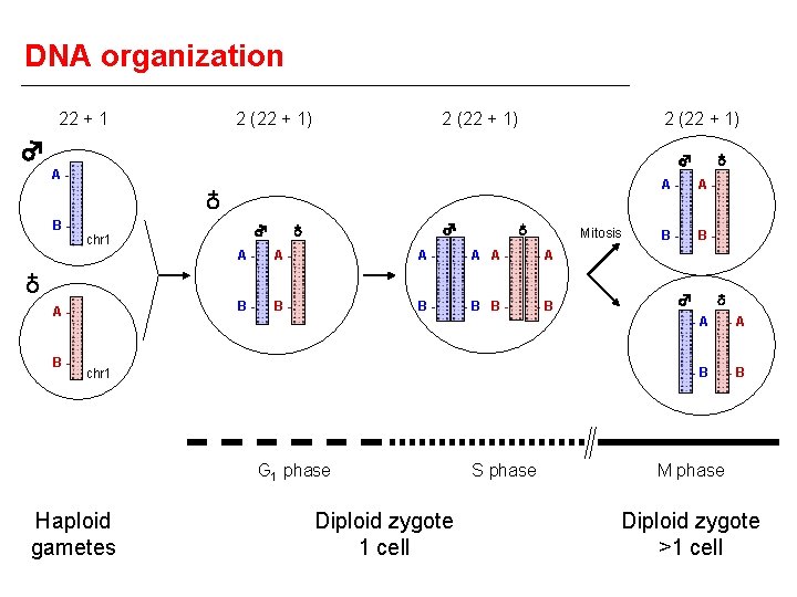
DNA organization 22 + 1 2 (22 + 1) ♂ ♁ B- chr 1 ♂ ♂ ♁ ♁ Mitosis A- A- A- -A B- B- B- -B ♁ A- B- ♁ ♂ A- chr 1 G 1 phase Haploid gametes Diploid zygote 1 cell S phase A- A- B- B- ♂ ♁ -A -A -B -B M phase Diploid zygote >1 cell

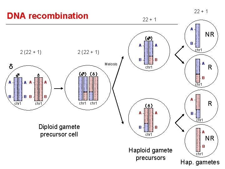
22 + 1 DNA recombination 22 + 1 A- NR (♂) A- 2 (22 + 1) -A chr 1 2 (22 + 1) BMeiosis ♁ ♂ -B -A chr 1 (♂) (♁) ♁ A- -A B- -B chr 1 B- chr 1 R -B chr 1 A- chr 1 R (♁) A- -A Bchr 1 Diploid gamete precursor cell B- -B chr 1 Haploid gamete precursors -A NR -B chr 1 Hap. gametes

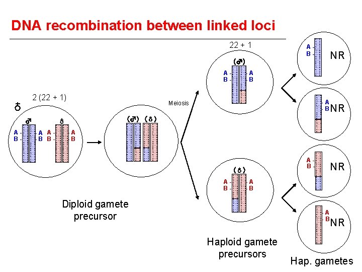
DNA recombination between linked loci 22 + 1 AB- NR (♂) AB- 2 (22 + 1) ♁ ♂ AB- -A -B Meiosis NR (♂) (♁) ♁ -A A-B B- -A -B AB- (♁) AB- NR -A -B Diploid gamete precursor -A -B Haploid gamete precursors NR Hap. gametes

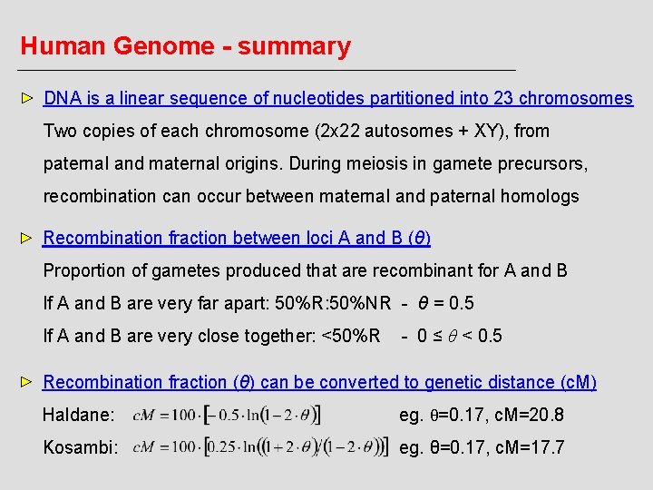
Human Genome - summary DNA is a linear sequence of nucleotides partitioned into 23 chromosomes Two copies of each chromosome (2 x 22 autosomes + XY), from paternal and maternal origins. During meiosis in gamete precursors, recombination can occur between maternal and paternal homologs Recombination fraction between loci A and B (θ) Proportion of gametes produced that are recombinant for A and B If A and B are very far apart: 50%R: 50%NR - θ = 0. 5 If A and B are very close together: <50%R - 0 ≤ θ < 0. 5 Recombination fraction (θ) can be converted to genetic distance (c. M) Haldane: eg. θ=0. 17, c. M=20. 8 Kosambi: eg. θ=0. 17, c. M=17. 7

3. Principles of Linkage Analysis

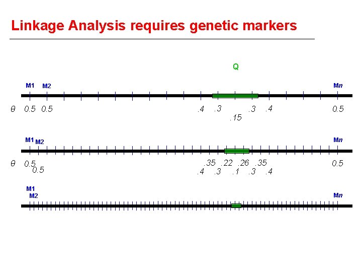
Linkage Analysis requires genetic markers Q M 1 θ Mn M 2 0. 5 . 4 . 3 . 15 . 3 . 4 M 1 M 2 θ 0. 5 M 1 M 2 0. 5 Mn . 35. 22. 26. 35. 4. 3. 1. 3. 4 0. 5 Mn

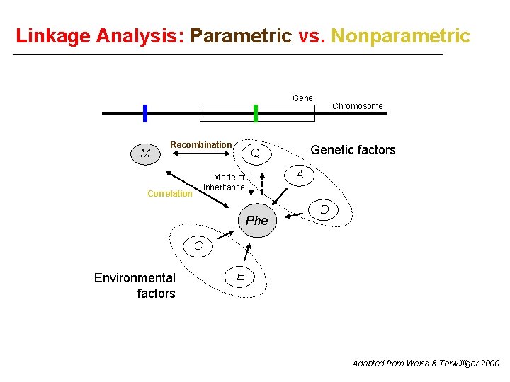
Linkage Analysis: Parametric vs. Nonparametric Gene M Recombination Genetic factors Q A Mode of inheritance Correlation Chromosome Phe D C Environmental factors E Adapted from Weiss & Terwilliger 2000

4. Parametric Linkage Analysis

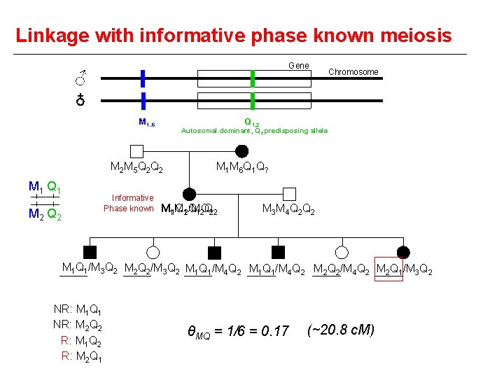
Linkage with informative phase known meiosis Gene ♂ ♁ M 1. . 6 Q 1, 2 Autosomal dominant, Q 1 predisposing allele M 2 M 5 Q 2 M 1 Q 1 Informative Phase known M 2 Q 2 Chromosome M 1 M 6 Q 1 Q ? Q 21 Q /M 12 QQ 22 M 1 M M 3 M 4 Q 2 M 1 Q 1/M 3 Q 2 M 2 Q 2/M 3 Q 2 M 1 Q 1/M 4 Q 2 M 2 Q 2/M 4 Q 2 M 2 Q 1/M 3 Q 2 NR: M 1 Q 1 NR: M 2 Q 2 R: M 1 Q 2 R: M 2 Q 1 θMQ = 1/6 = 0. 17 (~20. 8 c. M)

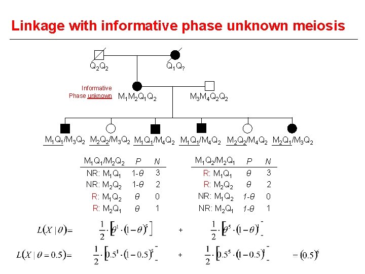
Linkage with informative phase unknown meiosis Q 2 Q 2 Informative Phase unknown Q 1 Q ? M 1 M 2 Q 1 Q 2 M 3 M 4 Q 2 M 1 Q 1/M 3 Q 2 M 2 Q 2/M 3 Q 2 M 1 Q 1/M 4 Q 2 M 2 Q 2/M 4 Q 2 M 2 Q 1/M 3 Q 2 M 1 Q 1/M 2 Q 2 NR: M 1 Q 1 NR: M 2 Q 2 R: M 1 Q 2 R: M 2 Q 1 P 1 -θ θ θ M 1 Q 2/M 2 Q 1 N 3 2 R: M 1 Q 1 R: M 2 Q 2 NR: M 1 Q 2 NR: M 2 Q 1 0 1 + + P θ θ 1 -θ N 3 2 0 1

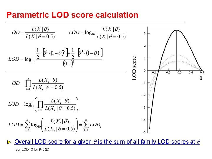
Parametric LOD score calculation Overall LOD score for a given θ is the sum of all family LOD scores at θ eg. LOD=3 for θ=0. 28

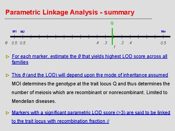
Parametric Linkage Analysis - summary Q M 1 θ Mn M 2 0. 5 . 4 . 3 . 1 . 3 . 4 0. 5 For each marker, estimate the θ that yields highest LOD score across all families This θ (and the LOD) will depend upon the mode of inheritance assumed MOI determines the genotype at the trait locus Q and thus determines the number of meiosis which are recombinant or nonrecombinant. Limited to Mendelian diseases. Markers with a significant parametric LOD score (>3) are said to be linked to the trait locus with recombination fraction θ

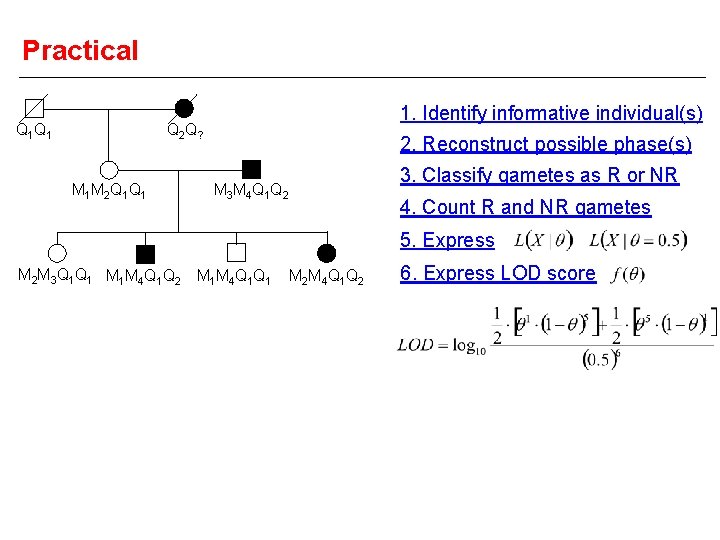
Practical Q 1 Q 1 1. Identify informative individual(s) Q 2 Q ? M 1 M 2 Q 1 2. Reconstruct possible phase(s) 3. Classify gametes as R or NR M 3 M 4 Q 1 Q 2 4. Count R and NR gametes 5. Express M 2 M 3 Q 1 M 1 M 4 Q 1 Q 2 M 1 M 4 Q 1 M 3 Q 1/M 4 Q 2 NR: M 3 Q 1 NR: M 4 Q 2 R: M 3 Q 2 R: M 4 Q 1 P 1 -θ θ θ N 1 2 0 1 6. Express LOD score M 2 M 4 Q 1 Q 2 M 3 Q 2/M 4 Q 1 R: M 3 Q 1 R: M 4 Q 2 NR: M 3 Q 2 NR: M 4 Q 1 P θ θ 1 -θ N 1 2 0 1 1 -θ + +

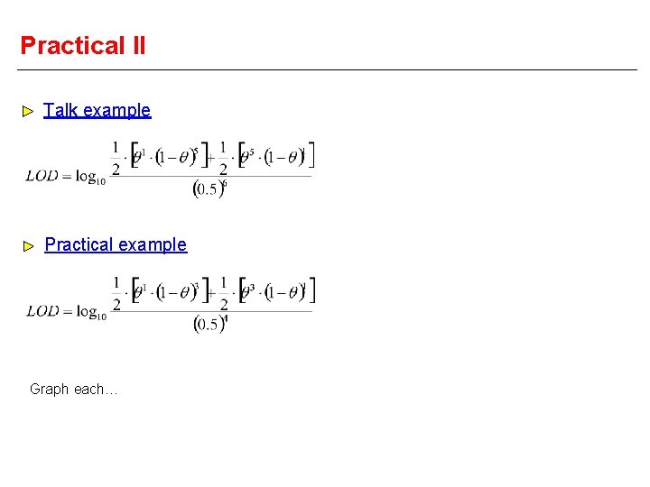
Practical II Talk example Practical example Graph each…

Outline 1. Aim 2. The Human Genome 3. Principles of Linkage Analysis 4. Parametric Linkage Analysis 5. Nonparametric Linkage Analysis

5. Nonparametric Linkage Analysis

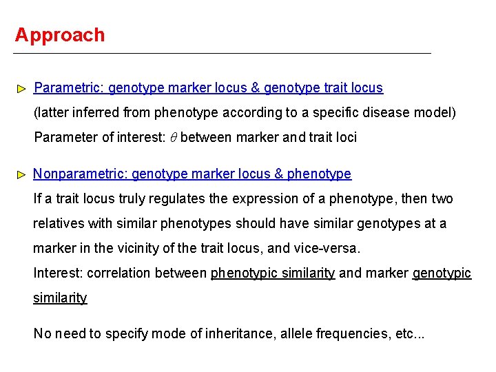
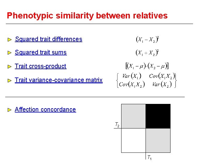
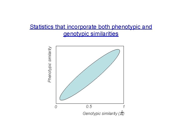
Approach Parametric: genotype marker locus & genotype trait locus (latter inferred from phenotype according to a specific disease model) Parameter of interest: θ between marker and trait loci Nonparametric: genotype marker locus & phenotype If a trait locus truly regulates the expression of a phenotype, then two relatives with similar phenotypes should have similar genotypes at a marker in the vicinity of the trait locus, and vice-versa. Interest: correlation between phenotypic similarity and marker genotypic similarity No need to specify mode of inheritance, allele frequencies, etc. . .

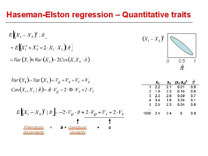
Phenotypic similarity between relatives Squared trait differences Squared trait sums Trait cross-product Trait variance-covariance matrix Affection concordance T 2 T 1

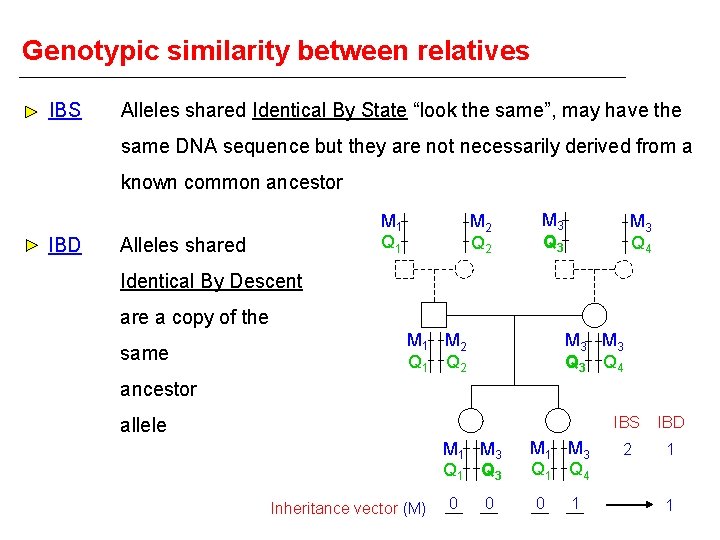
Genotypic similarity between relatives IBS Alleles shared Identical By State “look the same”, may have the same DNA sequence but they are not necessarily derived from a known common ancestor IBD M 1 Q 1 Alleles shared M 2 Q 2 M 3 Q 3 M 3 Q 4 Identical By Descent are a copy of the same M 1 M 2 Q 1 Q 2 M 3 Q 3 Q 4 ancestor allele M 1 M 3 Q 1 Q 3 Inheritance vector (M) 0 0 M 1 M 3 Q 1 Q 4 0 1 IBS IBD 2 1 1

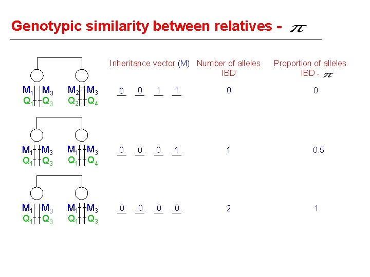
Genotypic similarity between relatives Inheritance vector (M) Number of alleles IBD Proportion of alleles IBD - M 1 M 3 Q 1 Q 3 M 2 M 3 Q 2 Q 4 0 0 1 1 0 0 M 1 M 3 Q 1 Q 3 M 1 M 3 Q 1 Q 4 0 0 0 1 1 0. 5 M 1 M 3 Q 1 Q 3 0 0 2 1

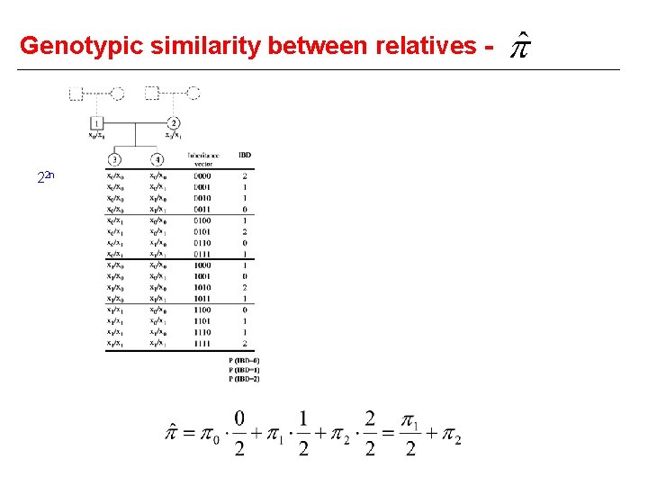
Genotypic similarity between relatives - 22 n

Phenotypic similarity Statistics that incorporate both phenotypic and genotypic similarities 0 0. 5 1 Genotypic similarity ( )

Haseman-Elston regression – Quantitative traits 0 Phenotypic dissimilarity = b × Genotypic similarity + c 0. 5 1

VC ML – Quantitative & Categorical traits method 0 H 1 : H 0 : e. g. LOD=3 0. 5 1

Genome-wide linkage analysis (e. g. VC) Individual LOD scores can be expressed as P values (Pointwise) LOD 2. 1 (x 4. 6) Chi-sq (n-df) 9. 67 P value 0. 0009

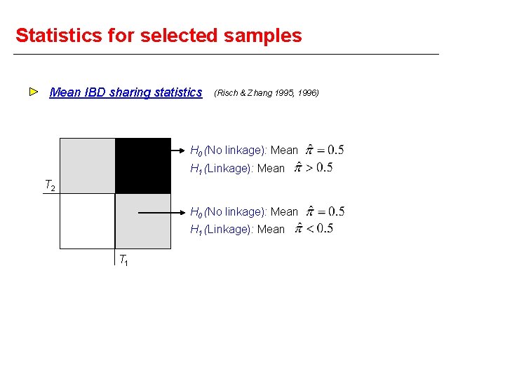
Statistics for selected samples Mean IBD sharing statistics (Risch & Zhang 1995, 1996) H 0 (No linkage): Mean H 1 (Linkage): Mean T 2 H 0 (No linkage): Mean H 1 (Linkage): Mean T 1

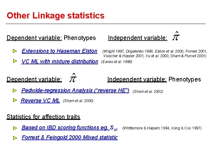
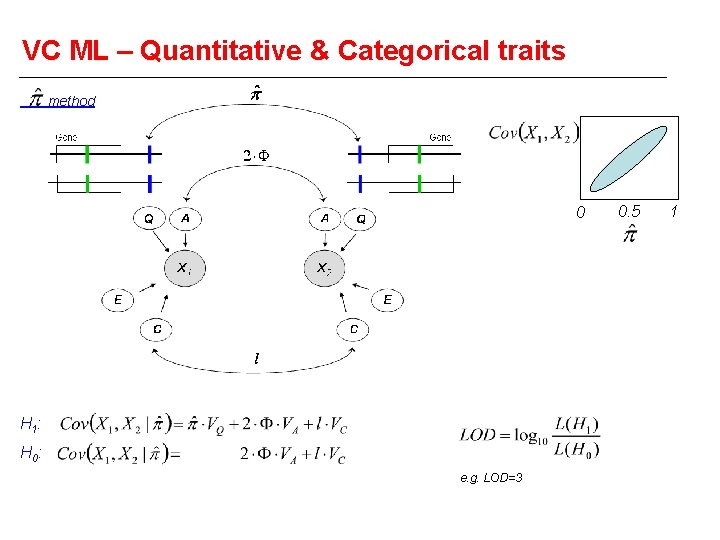
Other Linkage statistics Dependent variable: Phenotypes Extensions to Haseman Elston VC ML with mixture distribution Dependent variable: Independent variable: (Wright 1997, Drigalenko 1998, Elston et al. 2000, Forrest 2001, Visscher & Hopper 2001, Xu et al. 2000, Sham & Purcell 2001) (Eaves et al. 1996) Independent variable: Phenotypes Pedwide-regression Analysis (“reverse HE”) Reverse VC ML (Sham et al. 2002) (Sham et al. 2000) Statistics for affection traits Based on IBD scoring functions eg. Sall Forrest & Feingold 2000 Mixed statistic (Whittemore & Halpern 1994, Kong & Cox 1997)

Nonparametric Linkage Analysis - summary No need to specify mode of inheritance Models phenotypic and genotypic similarity of relatives Expression of phenotypic similarity, calculation of IBD HE and VC are the most popular statistics used for linkage of quantitative traits Other statistics available, specially for affection traits Type I error? Power?

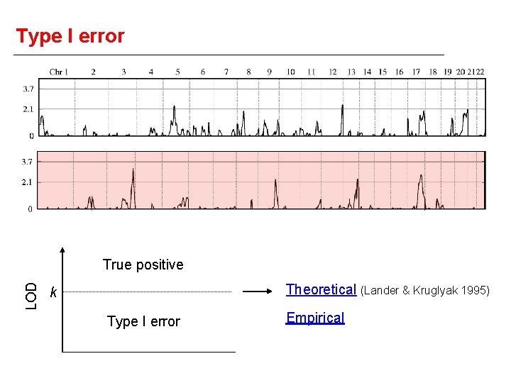
Type I error LOD True positive Theoretical (Lander & Kruglyak 1995) k Type I error Empirical

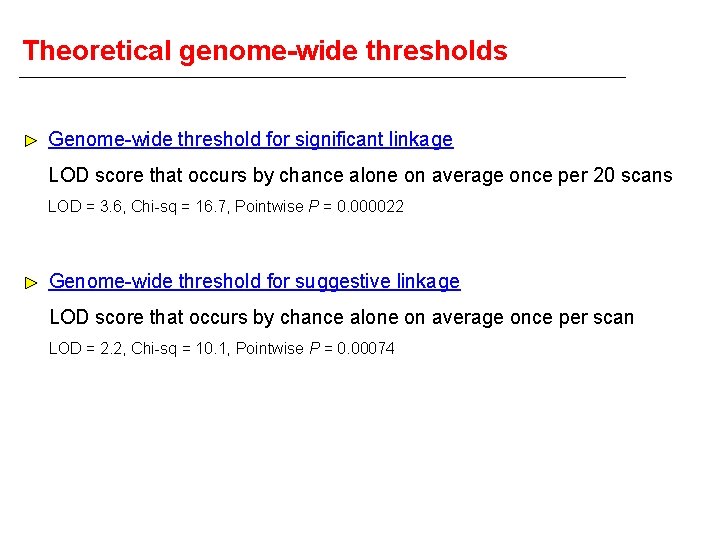
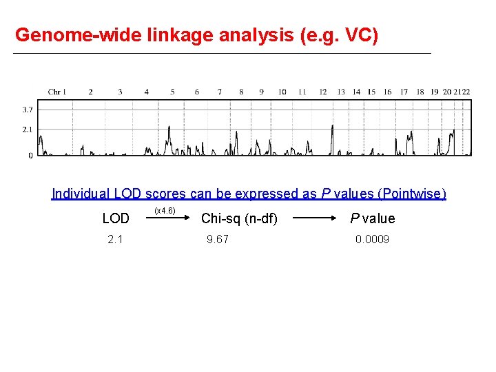
Theoretical genome-wide thresholds Genome-wide threshold for significant linkage LOD score that occurs by chance alone on average once per 20 scans LOD = 3. 6, Chi-sq = 16. 7, Pointwise P = 0. 000022 Genome-wide threshold for suggestive linkage LOD score that occurs by chance alone on average once per scan LOD = 2. 2, Chi-sq = 10. 1, Pointwise P = 0. 00074

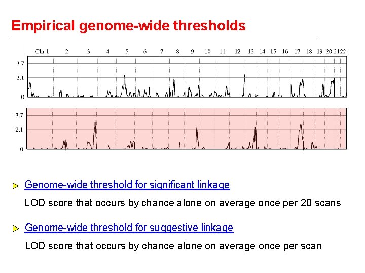
Empirical genome-wide thresholds Genome-wide threshold for significant linkage LOD score that occurs by chance alone on average once per 20 scans Genome-wide threshold for suggestive linkage LOD score that occurs by chance alone on average once per scan