Linear State Feedback Pole Placement State Estimation Integral

Linear State Feedback Pole Placement, State Estimation, Integral Control, LQR, Kalman Estimators M. V. Iordache, EEGR 4933 Automatic Control Systems, Spring 2019, Le. Tourneau University 1

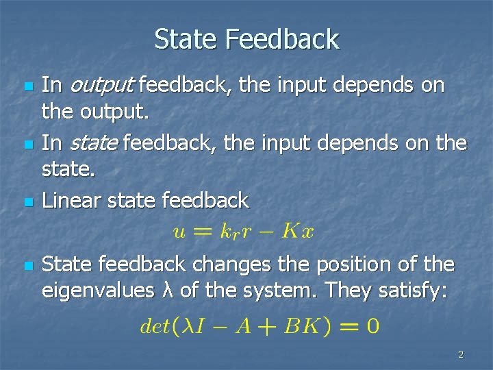
State Feedback n n In output feedback, the input depends on the output. In state feedback, the input depends on the state. Linear state feedback State feedback changes the position of the eigenvalues λ of the system. They satisfy: 2

State Feedback n 3

Ackerman’s Formula n 4

Pole Placement Limitations n n n Linear models are usually valid for small enough inputs. Actuators may not be able to apply the requested input if the desired response is too fast. Typically the state x cannot be measured directly state estimation. 5

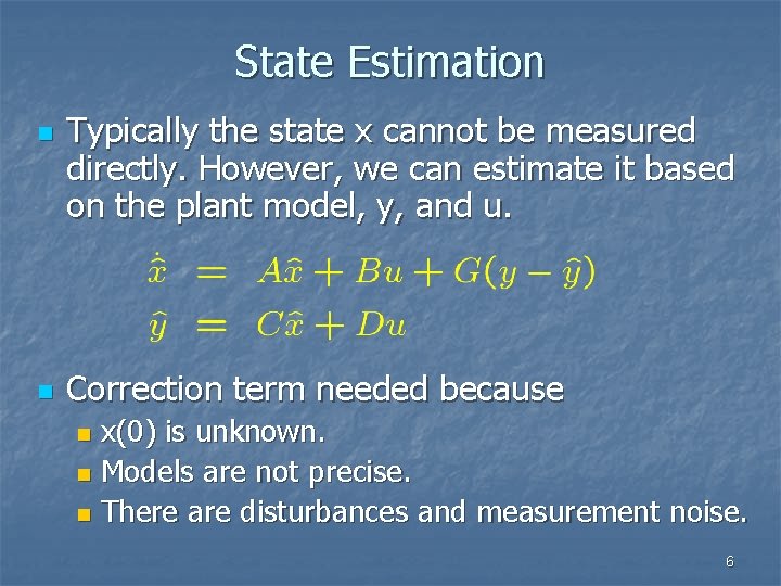
State Estimation n n Typically the state x cannot be measured directly. However, we can estimate it based on the plant model, y, and u. Correction term needed because x(0) is unknown. n Models are not precise. n There are disturbances and measurement noise. n 6

State Estimation n 7

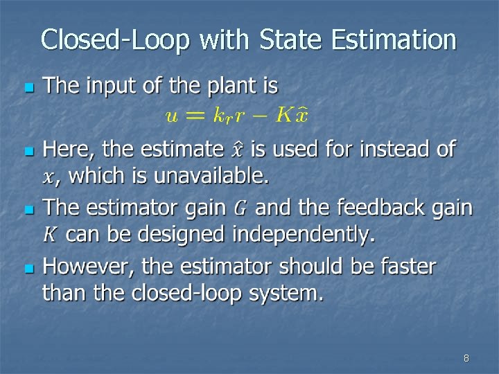
Closed-Loop with State Estimation n 8

Closed-Loop with State Estimation The textbook states that: n n n A rule of thumb often stated is to make the estimator two to four times faster than the system. State estimation can be dangerous, since the plant is controlled based on estimates and not actual state measurements. … great care must be exercised to ensure that the effects of the estimator are well understood for all possible conditions of system operation. 9

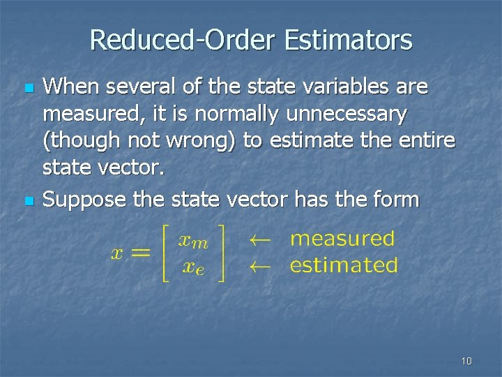
Reduced-Order Estimators n n When several of the state variables are measured, it is normally unnecessary (though not wrong) to estimate the entire state vector. Suppose the state vector has the form 10

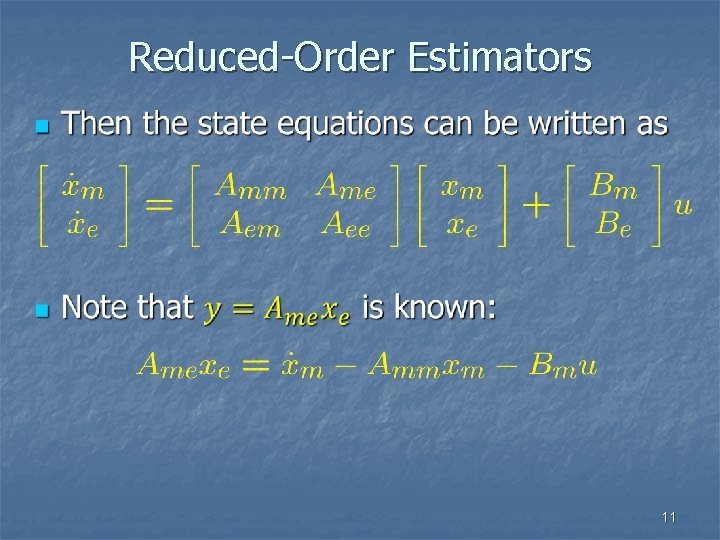
Reduced-Order Estimators n 11

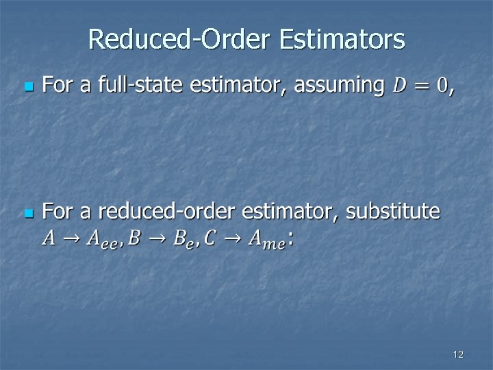
Reduced-Order Estimators n 12

Integral Control n n Generalizes the PI control to state variable models. Can be used to Track one or more references ri. n Reject constant disturbances. n 13

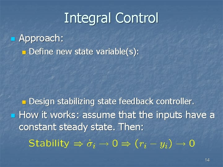
Integral Control n n Approach: n Define new state variable(s): n Design stabilizing state feedback controller. How it works: assume that the inputs have a constant steady state. Then: 14

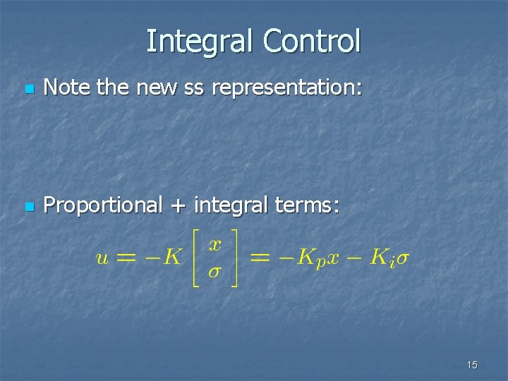
Integral Control n Note the new ss representation: n Proportional + integral terms: 15

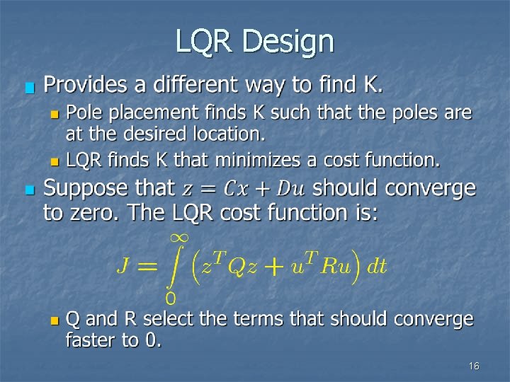
LQR Design n 16

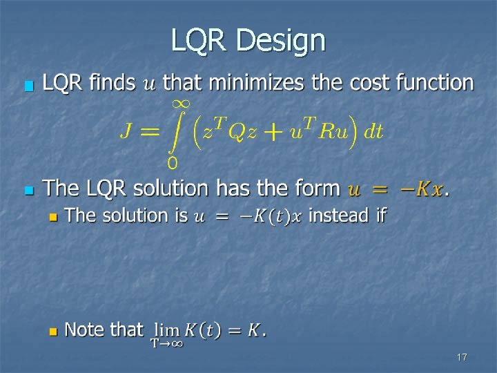
LQR Design n 17

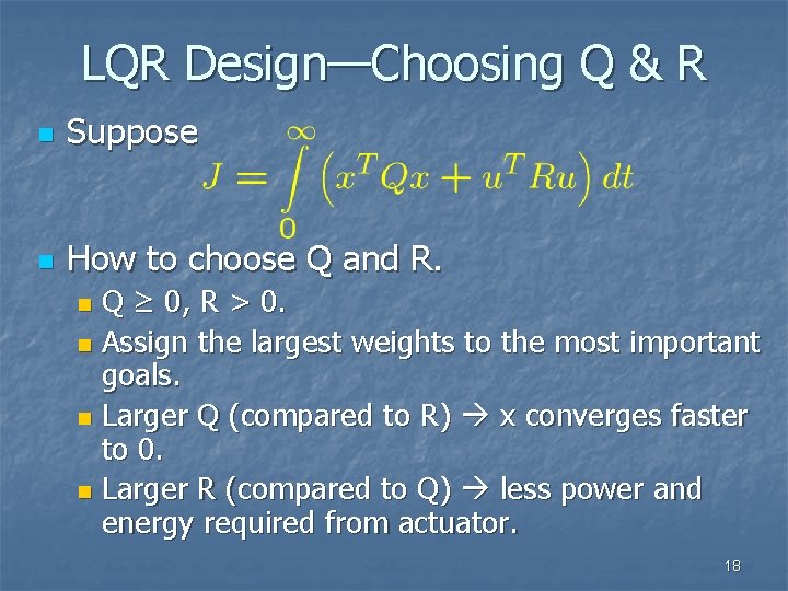
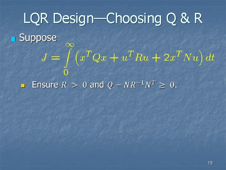
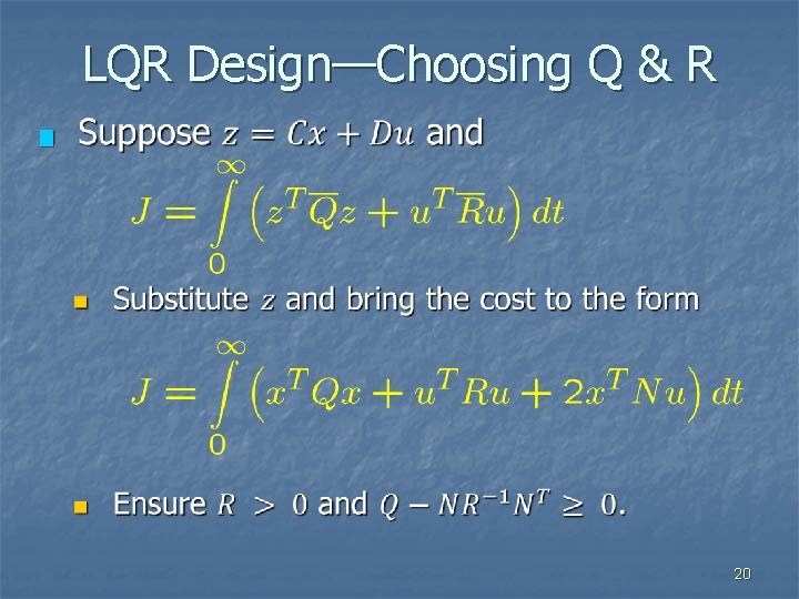
LQR Design—Choosing Q & R n Suppose n How to choose Q and R. Q ≥ 0, R > 0. n Assign the largest weights to the most important goals. n Larger Q (compared to R) x converges faster to 0. n Larger R (compared to Q) less power and energy required from actuator. n 18

LQR Design—Choosing Q & R n 19

LQR Design—Choosing Q & R n 20

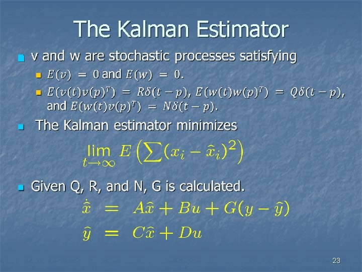
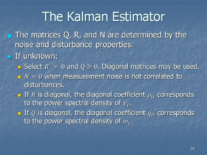
The Kalman Estimator n n n Real systems affected by noise (v) and disturbances (w): Since v and w are unknown, estimators always have some error. The Kalman estimator minimizes the error. 21

The Kalman Estimator n The pole placement method: Finds G that places poles at desired location. n Estimation error converges to zero assuming zero noise and disturbances. n n The Kalman estimator method: Finds G that minimizes estimation error. n The error is still zero for zero noise and disturbances. n The Kalman estimator is optimal under conditions that can be achieved only approximately in practice. n 22

The Kalman Estimator n 23

The Kalman Estimator n 24

LQG Design n n Use the Kalman estimator for the state estimate. Use the LQR design for the state feedback gain. If TF of plant is given, convert TF to a state space model. LQG and integral control can be combined. 25

Discrete-Time Methods n n n The continuous-time methods have straightforward extensions to discrete-time. We describe them briefly now. We will discuss them in more detail later. 26

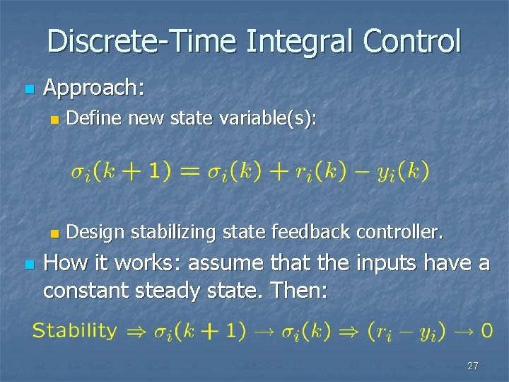
Discrete-Time Integral Control n n Approach: n Define new state variable(s): n Design stabilizing state feedback controller. How it works: assume that the inputs have a constant steady state. Then: 27

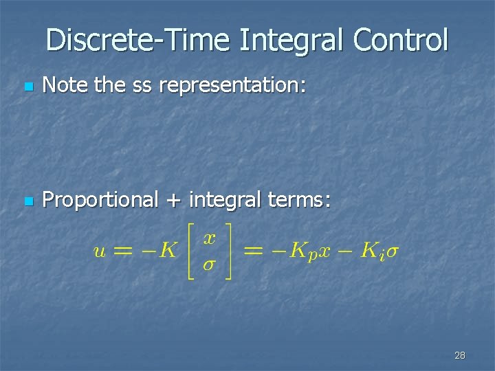
Discrete-Time Integral Control n Note the ss representation: n Proportional + integral terms: 28

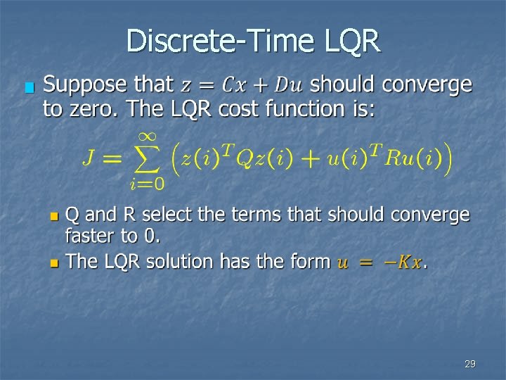
Discrete-Time LQR n 29

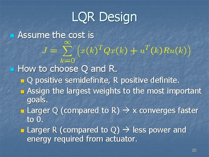
LQR Design n Assume the cost is n How to choose Q and R. Q positive semidefinite, R positive definite. n Assign the largest weights to the most important goals. n Larger Q (compared to R) x converges faster to 0. n Larger R (compared to Q) less power and energy required from actuator. n 30

Model Predictive Control n n n Optimal control is related to MPC: typically in the discrete-time setting. In MPC, the input u(k) is determined by solving an optimization problem at every time step. At time k, the control input u(k) is calculated based on measurements at time k and a model of the plant. The prediction horizon p indicates that the final time of the optimization problem is k+p. 31

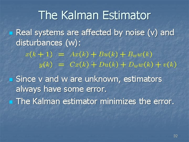
The Kalman Estimator n n n Real systems are affected by noise (v) and disturbances (w): Since v and w are unknown, estimators always have some error. The Kalman estimator minimizes the error. 32

The Kalman Estimator n The pole placement method: Finds G that places poles at desired location. n Estimation error converges to zero assuming zero noise and disturbances. n n The Kalman estimator method: Finds G that minimizes estimation error. n The error is still zero for zero noise and disturbances. n 33

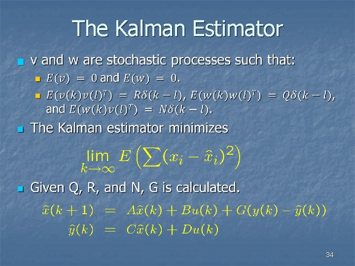
The Kalman Estimator n 34