Linear Sort Our intuition about the future is

Linear Sort "Our intuition about the future is linear. But the reality of information technology is exponential, and that makes a profound difference. If I take 30 steps linearly, I get to 30. If I take 30 steps exponentially, I get to a billion. " -Ray Kurzweil CLRS, Sections 8. 1 – 8. 3

Lower Bound for Sorting 8 All the sorting algorithms seen so far are called comparison sorts. – They sort by using comparison operations between the array elements. 8 We can show that any comparison sort must make Ω(n*log(n)) comparisons in the worst case to sort n elements. CS 321 - Data Structures 2

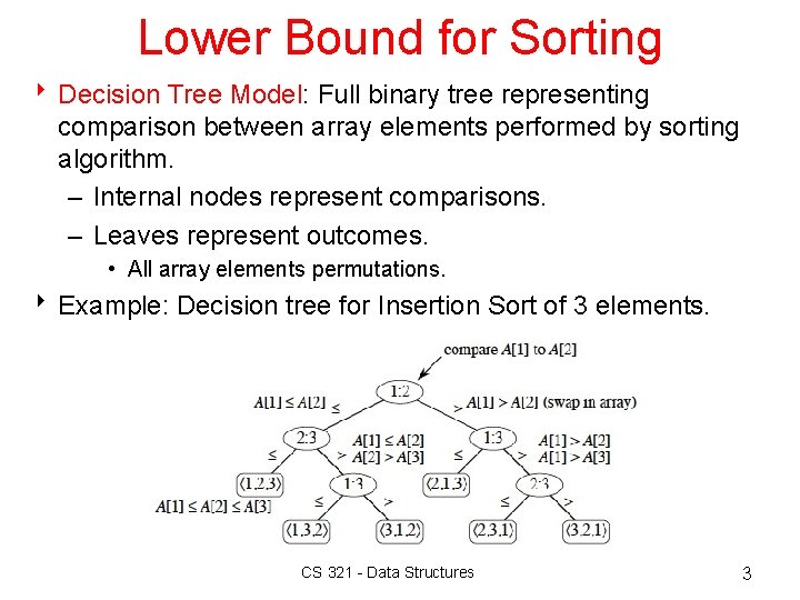
Lower Bound for Sorting 8 Decision Tree Model: Full binary tree representing comparison between array elements performed by sorting algorithm. – Internal nodes represent comparisons. – Leaves represent outcomes. • All array elements permutations. 8 Example: Decision tree for Insertion Sort of 3 elements. CS 321 - Data Structures 3

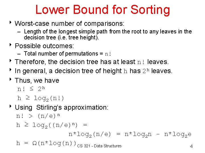
Lower Bound for Sorting 8 Worst-case number of comparisons: – Length of the longest simple path from the root to any leaves in the decision tree (i. e. tree height). 8 Possible outcomes: – Total number of permutations = n! 8 Therefore, the decision tree has at least n! leaves. 8 In general, a decision tree of height h has 2 h leaves. 8 Thus, we have n! ≤ 2 h h ≥ log 2(n!) 8 Using Stirling’s approximation: n! > (n/e)n h ≥ log 2((n/e)n) = n*log 2(n/e) = n*log 2 n - n*log 2 e h = Ω(n*log(n))CS 321 - Data Structures 4

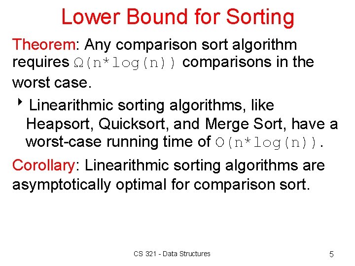
Lower Bound for Sorting Theorem: Any comparison sort algorithm requires Ω(n*log(n)) comparisons in the worst case. 8 Linearithmic sorting algorithms, like Heapsort, Quicksort, and Merge Sort, have a worst-case running time of O(n*log(n)). Corollary: Linearithmic sorting algorithms are asymptotically optimal for comparison sort. CS 321 - Data Structures 5

Can we do better? CS 321 - Data Structures 6

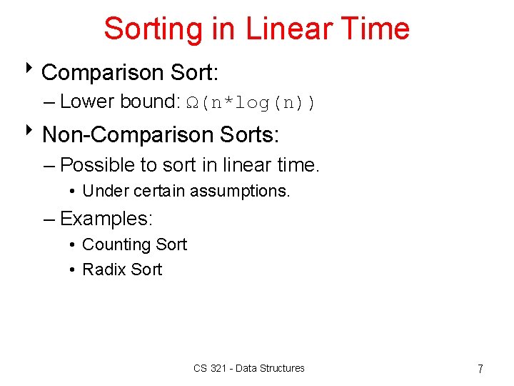
Sorting in Linear Time 8 Comparison Sort: – Lower bound: Ω(n*log(n)) 8 Non-Comparison Sorts: – Possible to sort in linear time. • Under certain assumptions. – Examples: • Counting Sort • Radix Sort CS 321 - Data Structures 7

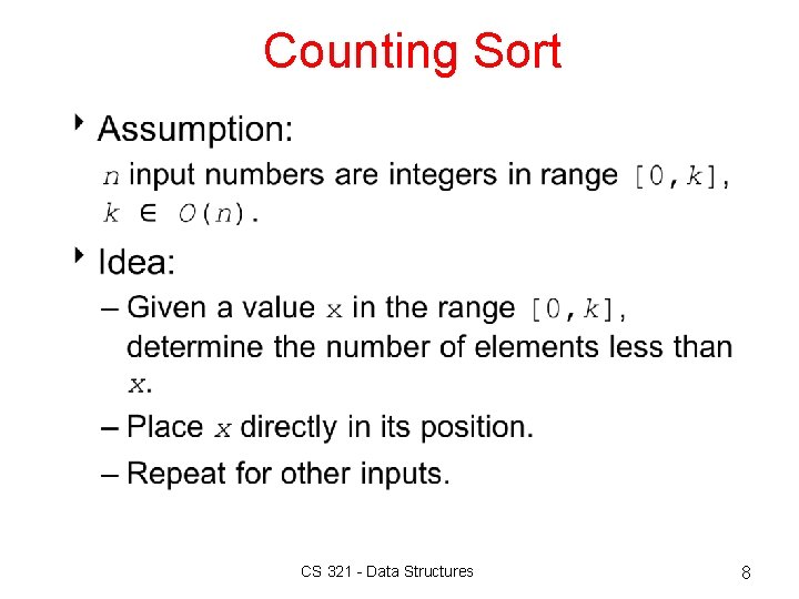
Counting Sort 8 CS 321 - Data Structures 8

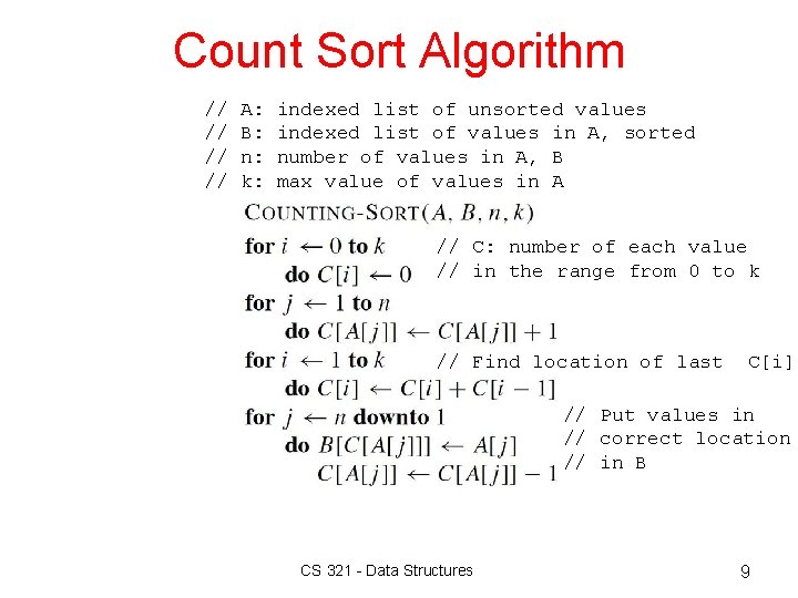
Count Sort Algorithm // // A: B: n: k: indexed list of unsorted values indexed list of values in A, sorted number of values in A, B max value of values in A // C: number of each value // in the range from 0 to k // Find location of last C[i] // Put values in // correct location // in B CS 321 - Data Structures 9

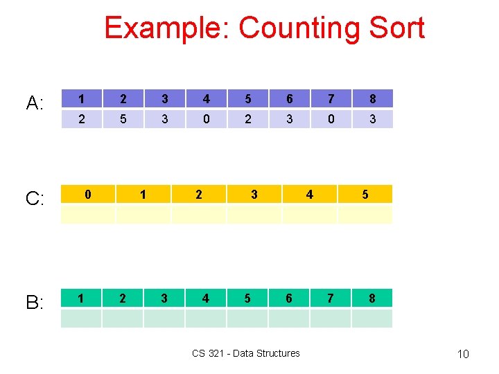
Example: Counting Sort A: C: B: 1 2 3 4 5 6 7 8 2 5 3 0 2 3 0 1 1 2 2 3 4 3 5 4 6 CS 321 - Data Structures 5 7 8 10

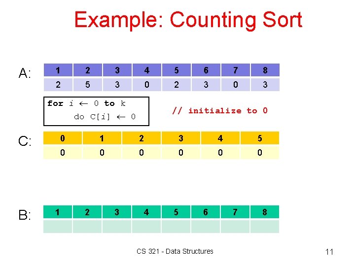
Example: Counting Sort A: 1 2 3 4 5 6 7 8 2 5 3 0 2 3 0 3 for i 0 to k // initialize to 0 do C[i] 0 C: B: 0 1 2 3 4 5 0 0 0 1 2 3 4 5 6 CS 321 - Data Structures 7 8 11

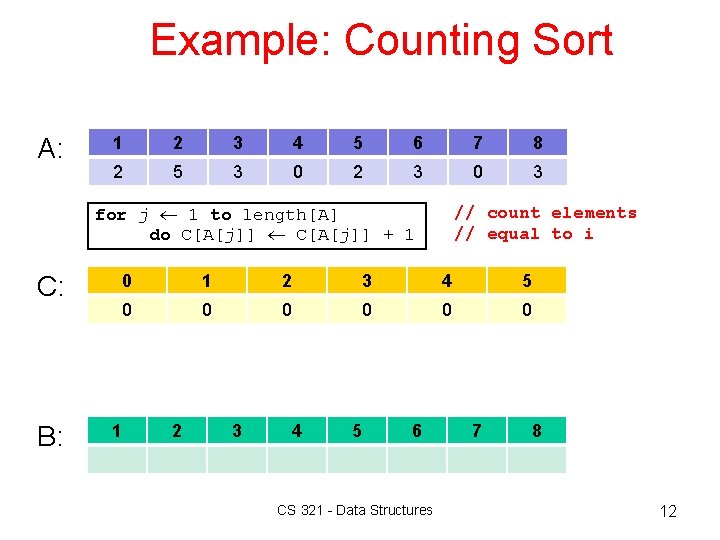
Example: Counting Sort A: 1 2 3 4 5 6 7 8 2 5 3 0 2 3 0 3 for j 1 to length[A] do C[A[j]] + 1 C: B: // count elements // equal to i 0 1 2 3 4 5 0 0 0 1 2 3 4 5 6 CS 321 - Data Structures 7 8 12

Example: Counting Sort A: 1 2 3 4 5 6 7 8 2 5 3 0 2 3 0 3 for j 1 to length[A] do C[A[j]] + 1 C: B: j = 1 C[2] 0 + 1 0 1 2 3 4 5 0 0 1 0 0 0 1 2 3 4 5 6 CS 321 - Data Structures 7 8 13

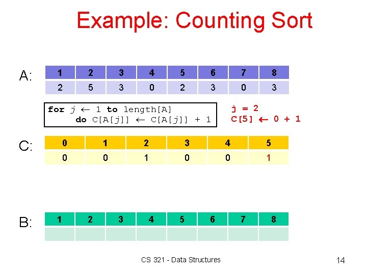
Example: Counting Sort A: 1 2 3 4 5 6 7 8 2 5 3 0 2 3 0 3 for j 1 to length[A] do C[A[j]] + 1 C: B: j = 2 C[5] 0 + 1 0 1 2 3 4 5 0 0 1 1 2 3 4 5 6 CS 321 - Data Structures 7 8 14

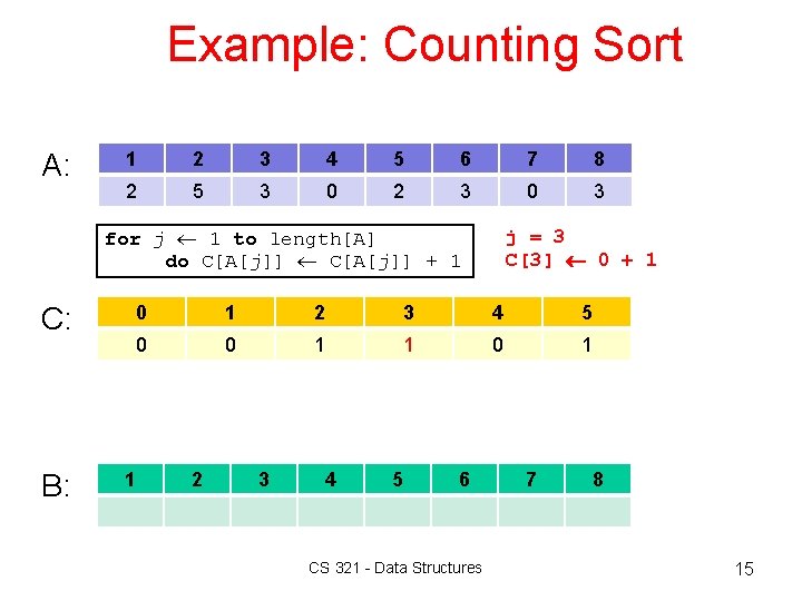
Example: Counting Sort A: 1 2 3 4 5 6 7 8 2 5 3 0 2 3 0 3 for j 1 to length[A] do C[A[j]] + 1 C: B: j = 3 C[3] 0 + 1 0 1 2 3 4 5 0 0 1 1 2 3 4 5 6 CS 321 - Data Structures 7 8 15

Example: Counting Sort A: 1 2 3 4 5 6 7 8 2 5 3 0 2 3 0 3 for j 1 to length[A] do C[A[j]] + 1 C: B: j = 4 C[0] 0 + 1 0 1 2 3 4 5 1 0 1 1 2 3 4 5 6 CS 321 - Data Structures 7 8 16

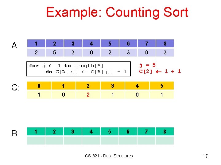
Example: Counting Sort A: 1 2 3 4 5 6 7 8 2 5 3 0 2 3 0 3 for j 1 to length[A] do C[A[j]] + 1 C: B: j = 5 C[2] 1 + 1 0 1 2 3 4 5 1 0 2 1 0 1 1 2 3 4 5 6 CS 321 - Data Structures 7 8 17

Example: Counting Sort A: 1 2 3 4 5 6 7 8 2 5 3 0 2 3 0 3 for j 1 to length[A] do C[A[j]] + 1 C: B: j = 6 C[3] 1 + 1 0 1 2 3 4 5 1 0 2 2 0 1 1 2 3 4 5 6 CS 321 - Data Structures 7 8 18

Example: Counting Sort A: 1 2 3 4 5 6 7 8 2 5 3 0 2 3 0 3 for j 1 to length[A] do C[A[j]] + 1 C: B: j = 7 C[0] 1 + 1 0 1 2 3 4 5 2 0 2 2 0 1 1 2 3 4 5 6 CS 321 - Data Structures 7 8 19

Example: Counting Sort A: 1 2 3 4 5 6 7 8 2 5 3 0 2 3 0 3 for j 1 to length[A] do C[A[j]] + 1 C: B: j = 8 C[0] 2 + 1 0 1 2 3 4 5 2 0 2 3 0 1 1 2 3 4 5 6 CS 321 - Data Structures 7 8 20

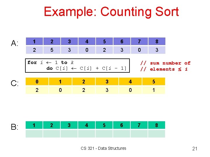
Example: Counting Sort A: 1 2 3 4 5 6 7 8 2 5 3 0 2 3 0 3 for i 1 to k do C[i] + C[i - 1] C: B: // sum number of // elements i 0 1 2 3 4 5 2 0 2 3 0 1 1 2 3 4 5 6 CS 321 - Data Structures 7 8 21

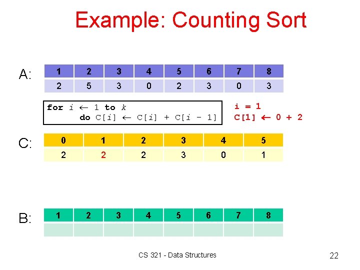
Example: Counting Sort A: 1 2 3 4 5 6 7 8 2 5 3 0 2 3 0 3 for i 1 to k do C[i] + C[i - 1] C: B: i = 1 C[1] 0 + 2 0 1 2 3 4 5 2 2 2 3 0 1 1 2 3 4 5 6 CS 321 - Data Structures 7 8 22

Example: Counting Sort A: 1 2 3 4 5 6 7 8 2 5 3 0 2 3 0 3 for i 1 to k do C[i] + C[i - 1] C: B: i = 2 C[2] 2 + 2 0 1 2 3 4 5 2 2 4 3 0 1 1 2 3 4 5 6 CS 321 - Data Structures 7 8 23

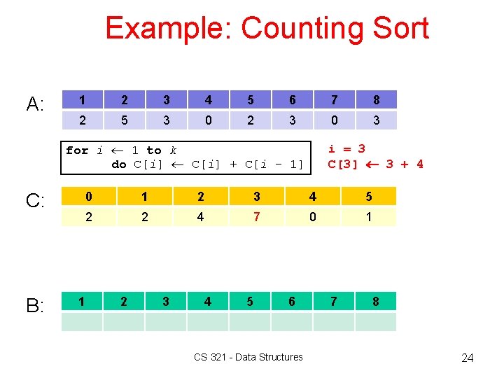
Example: Counting Sort A: 1 2 3 4 5 6 7 8 2 5 3 0 2 3 0 3 for i 1 to k do C[i] + C[i - 1] C: B: i = 3 C[3] 3 + 4 0 1 2 3 4 5 2 2 4 7 0 1 1 2 3 4 5 6 CS 321 - Data Structures 7 8 24

Example: Counting Sort A: 1 2 3 4 5 6 7 8 2 5 3 0 2 3 0 3 for i 1 to k do C[i] + C[i - 1] C: B: i = 4 C[4] 0 + 7 0 1 2 3 4 5 2 2 4 7 7 1 1 2 3 4 5 6 CS 321 - Data Structures 7 8 25

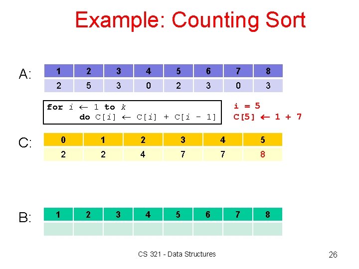
Example: Counting Sort A: 1 2 3 4 5 6 7 8 2 5 3 0 2 3 0 3 for i 1 to k do C[i] + C[i - 1] C: B: i = 5 C[5] 1 + 7 0 1 2 3 4 5 2 2 4 7 7 8 1 2 3 4 5 6 CS 321 - Data Structures 7 8 26

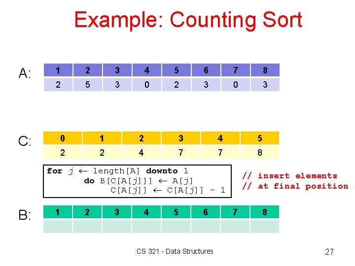
Example: Counting Sort A: C: 1 2 3 4 5 6 7 8 2 5 3 0 2 3 0 1 2 3 4 5 2 2 4 7 7 8 for j length[A] downto 1 do B[C[A[j]]] A[j] C[A[j]] - 1 B: 1 2 3 4 5 6 CS 321 - Data Structures // insert elements // at final position 7 8 27

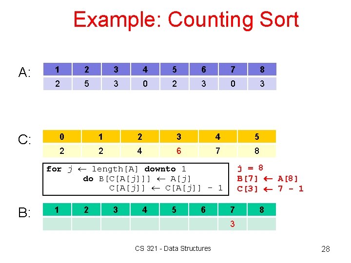
Example: Counting Sort A: C: 1 2 3 4 5 6 7 8 2 5 3 0 2 3 0 1 2 3 4 5 2 2 4 6 7 8 for j length[A] downto 1 do B[C[A[j]]] A[j] C[A[j]] - 1 B: 1 2 3 4 5 6 j = 8 B[7] A[8] C[3] 7 - 1 7 8 3 CS 321 - Data Structures 28

Example: Counting Sort A: C: 1 2 3 4 5 6 7 8 2 5 3 0 2 3 0 1 2 3 4 5 1 2 4 6 7 8 for j length[A] downto 1 do B[C[A[j]]] A[j] C[A[j]] - 1 B: 1 2 3 4 5 6 0 j = 7 B[2] A[7] C[0] 2 - 1 7 8 3 CS 321 - Data Structures 29

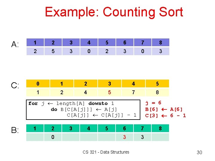
Example: Counting Sort A: C: 1 2 3 4 5 6 7 8 2 5 3 0 2 3 0 1 2 3 4 5 1 2 4 5 7 8 for j length[A] downto 1 do B[C[A[j]]] A[j] C[A[j]] - 1 B: 1 2 0 3 4 5 j = 6 B[6] A[6] C[3] 6 - 1 6 7 3 3 CS 321 - Data Structures 8 30

Example: Counting Sort A: C: 1 2 3 4 5 6 7 8 2 5 3 0 2 3 0 1 2 3 4 5 1 2 3 5 7 8 for j length[A] downto 1 do B[C[A[j]]] A[j] C[A[j]] - 1 B: 1 2 0 3 4 2 5 j = 5 B[4] A[5] C[2] 4 - 1 6 7 3 3 CS 321 - Data Structures 8 31

Example: Counting Sort A: C: 1 2 3 4 5 6 7 8 2 5 3 0 2 3 0 1 2 3 4 5 0 2 3 5 7 8 for j length[A] downto 1 do B[C[A[j]]] A[j] C[A[j]] - 1 B: 1 2 0 0 3 4 2 5 j = 4 B[1] A[4] C[0] 1 - 1 6 7 3 3 CS 321 - Data Structures 8 32

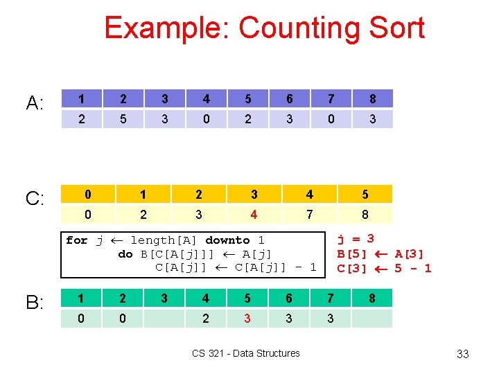
Example: Counting Sort A: C: 1 2 3 4 5 6 7 8 2 5 3 0 2 3 0 1 2 3 4 5 0 2 3 4 7 8 for j length[A] downto 1 do B[C[A[j]]] A[j] C[A[j]] - 1 B: 1 2 0 0 3 j = 3 B[5] A[3] C[3] 5 - 1 4 5 6 7 2 3 3 3 CS 321 - Data Structures 8 33

Example: Counting Sort A: C: 1 2 3 4 5 6 7 8 2 5 3 0 2 3 0 1 2 3 4 5 0 2 3 4 7 7 for j length[A] downto 1 do B[C[A[j]]] A[j] C[A[j]] - 1 B: 1 2 0 0 3 j = 2 B[8] A[2] C[3] 8 - 1 4 5 6 7 8 2 3 3 3 5 CS 321 - Data Structures 34

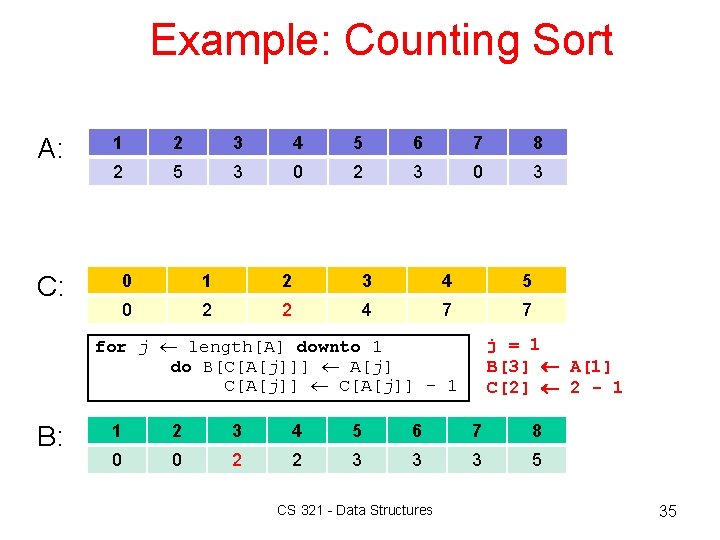
Example: Counting Sort A: C: 1 2 3 4 5 6 7 8 2 5 3 0 2 3 0 1 2 3 4 5 0 2 2 4 7 7 for j length[A] downto 1 do B[C[A[j]]] A[j] C[A[j]] - 1 B: j = 1 B[3] A[1] C[2] 2 - 1 1 2 3 4 5 6 7 8 0 0 2 2 3 3 3 5 CS 321 - Data Structures 35

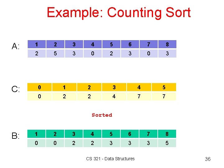
Example: Counting Sort A: C: 1 2 3 4 5 6 7 8 2 5 3 0 2 3 0 1 2 3 4 5 0 2 2 4 7 7 Sorted B: 1 2 3 4 5 6 7 8 0 0 2 2 3 3 3 5 CS 321 - Data Structures 36

Analysis of Count Sort COUNTING-SORT(A, B, k) for i 0 to k [Loop 1] Loops 1 and 3 do C[i] 0 takes Θ(k) time for j 1 to length[A] [Loop 2] do C[A[j]] + 1 // C[i] contains number of elements equal to Loops 2 and 4 i. takes Θ(n) time for i 1 to k [Loop 3] do C[i] + C[i - 1] // C[i] contains number of elements i. for j length[A] downto 1 [Loop 4] do B[C[A[j]]] A[j] C[A[j]] – 1 Total cost is (k+n). If k = O(n), then total cost is (n). CS 321 - Data Structures 37

Radix Sort 8 Radix Sort dates back as far as 1887. – Herman Hollerith used technique in tabulating machines. – The 1880 U. S. census took 7 years to complete. – With Hollerith's "tabulating machines, " the 1890 census took the Census Bureau six weeks. 8 Radix sort is another non-comparative sorting algorithm. – Sorts data with integer keys with d digits. – Sort least significant digits first, then sort the 2 nd one, then the 3 rd one, etc. , up to d digits. CS 321 - Data Structures 38

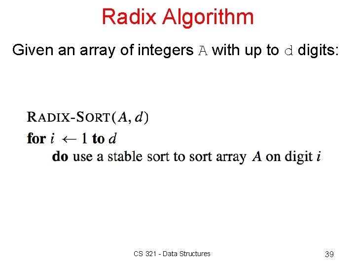
Radix Algorithm Given an array of integers A with up to d digits: CS 321 - Data Structures 39

Stable Sorting 8 Stability is a property of sorts. – If a sort guarantees the relative order of equal items stays the same, then it is a stable sort. – For instance: • [71, 6, 72, 5, 1, 2, 73, -5] – subscripts added for clarity • [-5, 1, 2, 5, 6, 71, 72, 73] – result of stable sort 8 Real world examples: – Sort playing cards by suit, then by value. – Sort people by state of residence, then by city. CS 321 - Data Structures 40

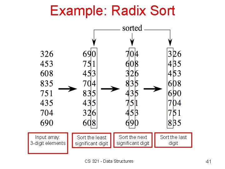
Example: Radix Sort Input array: 3 -digit elements Sort the least significant digit Sort the next significant digit CS 321 - Data Structures Sort the last digit 41

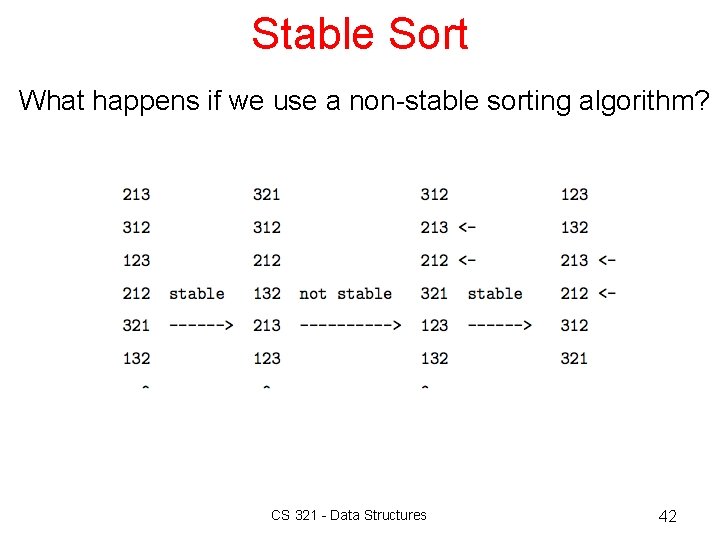
Stable Sort What happens if we use a non-stable sorting algorithm? CS 321 - Data Structures 42

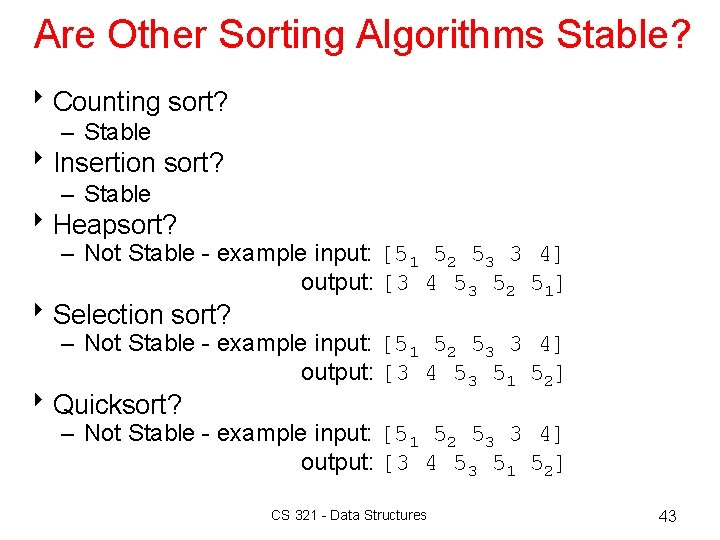
Are Other Sorting Algorithms Stable? 8 Counting sort? – Stable 8 Insertion sort? – Stable 8 Heapsort? – Not Stable - example input: [51 52 53 3 4] output: [3 4 53 52 51] 8 Selection sort? – Not Stable - example input: [51 52 53 3 4] output: [3 4 53 51 52] 8 Quicksort? – Not Stable - example input: [51 52 53 3 4] output: [3 4 53 51 52] CS 321 - Data Structures 43

Radix Sort for Non-Integers 8 Suppose a group of people, with last name, middle, and first name. 8 Sort it by the last name, then by middle, finally by the first name 8 Then after every pass of sort, the bins can be combined as one file and proceed to the next sort. CS 321 - Data Structures 44

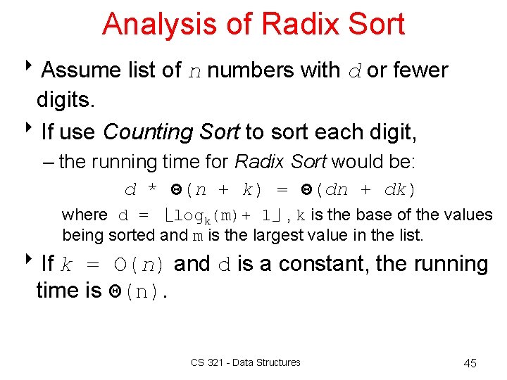
Analysis of Radix Sort 8 Assume list of n numbers with d or fewer digits. 8 If use Counting Sort to sort each digit, – the running time for Radix Sort would be: d * Θ(n + k) = Θ(dn + dk) where d = ⎿logk(m)+ 1⏌, k is the base of the values being sorted and m is the largest value in the list. 8 If k = O(n) and d is a constant, the running time is Θ(n). CS 321 - Data Structures 45

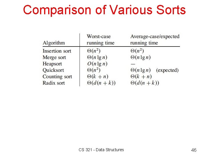
Comparison of Various Sorts CS 321 - Data Structures 46

CS 321 - Data Structures 47

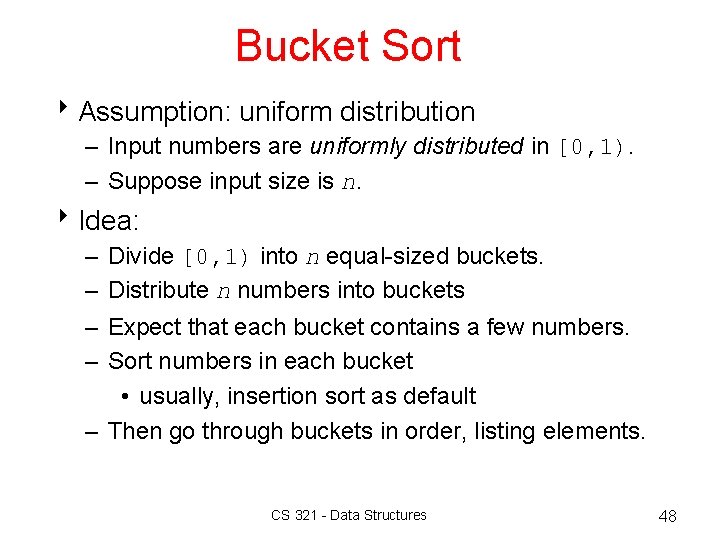
Bucket Sort 8 Assumption: uniform distribution – Input numbers are uniformly distributed in [0, 1). – Suppose input size is n. 8 Idea: – – Divide [0, 1) into n equal-sized buckets. Distribute n numbers into buckets Expect that each bucket contains a few numbers. Sort numbers in each bucket • usually, insertion sort as default – Then go through buckets in order, listing elements. CS 321 - Data Structures 48

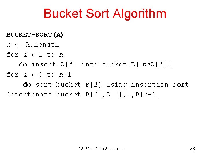
Bucket Sort Algorithm BUCKET-SORT(A) n A. length for i 1 to n do insert A[i] into bucket B[ n*A[i] ] for i 0 to n-1 do sort bucket B[i] using insertion sort Concatenate bucket B[0], B[1], …, B[n-1] CS 321 - Data Structures 49

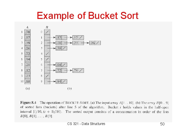
Example of Bucket Sort CS 321 - Data Structures 50

Analysis of Bucket Sort BUCKET-SORT(A) n length[A] for i 1 to n do insert A[i] into bucket B[ n. A[i] ] for i 0 to n-1 do sort bucket B[i] with insertion sort Concatenate bucket B[0], B[1], …, B[n-1] (1) O(n) O(ni 2) O(n) Where ni is the size of bucket B[i]. Thus, T(n) = (n) + i=0 n-1 O(ni 2) = (n) + n*O(2 -1/n) = (n) CS 321 - Data Structures 51

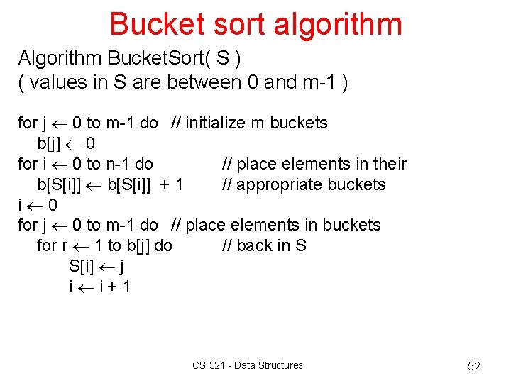
Bucket sort algorithm Algorithm Bucket. Sort( S ) ( values in S are between 0 and m-1 ) for j 0 to m-1 do // initialize m buckets b[j] 0 for i 0 to n-1 do // place elements in their b[S[i]] + 1 // appropriate buckets i 0 for j 0 to m-1 do // place elements in buckets for r 1 to b[j] do // back in S S[i] j i i+1 CS 321 - Data Structures 52

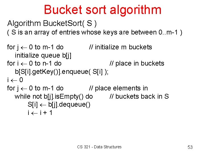
Bucket sort algorithm Algorithm Bucket. Sort( S ) ( S is an array of entries whose keys are between 0. . m-1 ) for j 0 to m-1 do // initialize m buckets initialize queue b[j] for i 0 to n-1 do // place in buckets b[S[i]. get. Key()]. enqueue( S[i] ); i 0 for j 0 to m-1 do // place elements in while not b[j]. is. Empty() do // buckets back in S S[i] b[j]. dequeue() i i+1 CS 321 - Data Structures 53

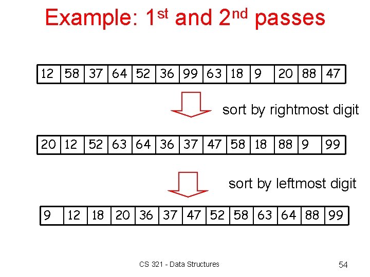
Example: 1 st and 2 nd passes 12 58 37 64 52 36 99 63 18 9 20 88 47 sort by rightmost digit 20 12 52 63 64 36 37 47 58 18 88 9 99 sort by leftmost digit 9 12 18 20 36 37 47 52 58 63 64 88 99 CS 321 - Data Structures 54

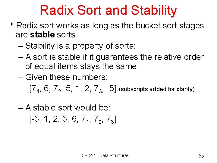
Radix Sort and Stability 8 Radix sort works as long as the bucket sort stages are stable sorts – Stability is a property of sorts: – A sort is stable if it guarantees the relative order of equal items stays the same – Given these numbers: [71, 6, 72, 5, 1, 2, 73, -5] (subscripts added for clarity) – A stable sort would be: [-5, 1, 2, 5, 6, 71, 72, 73] CS 321 - Data Structures 55