Linear regression Stats Club Marnie Brennan Have you

Linear regression Stats Club Marnie Brennan

Have you used any type of regression before?

References • Petrie and Sabin - Medical Statistics at a Glance: Chapter 27 & 28 Good • Petrie and Watson - Statistics for Veterinary and Animal Science: Pages 127 -140 Good • Dohoo, Martin and Stryhn – Veterinary Epidemiologic Research: Chapter 14

What is regression? • Use it to look at the relationship between variables – To see if one variable can be explained by another/several, or to see if one variable predicts the other • Linear regression – to look at the relationship between continuous (numerical) variables – This describes the linear relationship between two variables – You can determine the ‘line of best fit’ to describe the relationship – Our focus for today!

When would you use regression? • To determine if certain outcomes are associated with certain explanatory variables – Risk factors for disease • To determine if certain variables can ‘predict’ an outcome variable • Other reasons? ?

Single linear regression versus multiple linear regression • Simple/univariable linear regression – A single factor affecting a single outcome • Multiple/multivariable linear regression – Several factors affecting a single outcome – Can have binary, nominal and ordinal explanatory variables • With some manipulations e. g. creating dummy variables – We won’t focus on this today!

First step – descriptive stats • Scatter plot • What does the relationship look like between the two variables? • Calculate, using an equation, the regression line – the line that best suits the data • E. g. the minimisation between our actual values, and some predicted values that are created from the regression line

Scatter plot Taken from Petrie and Watson

Regression line Taken from Petrie and Watson

Regression equation (this is it for equations, I promise!) • Y = a + bx • Y = outcome variable • a = point at which the regression line crosses the Y axis • b = slope of the regression line – How much the average value of Y varies with each unit change in x • x = explanatory variable used to predict y

Creation of the regression line • Minimisation of residuals – Residual = The difference between an observed and predicted value • Residual = Observed value – fitted value – Aiming to minimise the sum of the squared deviations (residuals) between the line, and your points – Terminology = Method of least squares OR Ordinary least squares – You can put confidence intervals around the regression line (indicates the appropriateness of fit)

Regression line Residuals Taken from Petrie and Watson

What are the assumptions that have to be satisfied? • There is a linear relationship between x and y • X is measured without error • There is not multiple data from the same subjects (independence) • For each value of x, there is a distribution of values of y in the population, and this distribution is Normal • The variability of the distribution of the y values is the same for all values of x e. g. the variance is constant

Determining if we meet our assumptions • Residuals! No relationship apparent in the diagram = linear relationship assumption met Outcome variable Distribution of residuals is approximately Normal = Normality met Taken from Petrie and Watson

Determining if we meet our assumptions • Residuals! No tendency for the residuals to increase or decrease systematically with fitted values = constant variance assumption met Taken from Petrie and Watson

What if our assumptions cannot be met? • There is a linear relationship between x and y – Can try and transform the data e. g. logarithmic – If outliers are a problem: • Rule of thumb – if the outliers are outside +/-2 standard deviations away from the group mean, you can remove them, OR • If the point has a greater leverage than 4/n (n=number of pairs of observations), it should be investigated further • Run the analysis, remove the outliers and re-run the analysis – See if there is any difference • Other ways e. g. Cook’s distance

Outliers Taken from Shelton et al. (2012) Journal of Agricultural Science Vol 150

What if our assumptions cannot be met? • X is measured without error • There is not multiple data from the same subjects (independence) • The variability of the distribution of the y values is the same for all values of x e. g. the variance is constant • For each value of x, there is a distribution of values of y in the population, and this distribution is Normal – For the previous two points: • If there are moderate departures from these assumptions, we can potentially proceed with the analysis, but – The estimates of the standard errors and the p-values may be affected – This is quite vague and not necessarily useful!

How good is the model? • ANOVA table and residual variance (F-ratio) – Investigating the slope • Testing the null hypothesis that the true slope is zero • Examine the F-ratio in the ANOVA table – is the ratio of how good the model is to how bad it is • Calculate the test statistic (P-value is given) – if small, means that unlikely to get this F value (large) if the null hypothesis was true – A good model will have a large F-ratio (at least greater than 1)

Assessing how well the predictor explains the outcome • R 2 value (square of the correlation coefficient) = Coefficient of determination – The percentage of the variability of y that can be explained by its relationship with x – E. g. R 2 = 0. 33; 33% of the variation is explained by the variables within the analysis – 100 -R 2 is equal to the unexplained variance • Adjusted R 2 value – Accounts for the number of variables included in the model • Important for multiple linear regression

Other analyses • Additional things to consider: – Model ‘validation’ • Do they show that they explain what they seek to explain – Different ways of doing this e. g. using a proportion of the data and using the other proportion for testing

Minitab Or via Regression, Regression

Minitab

SPSS

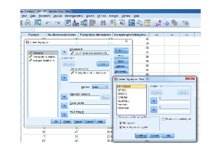
SPSS R 2 = The individual contribution of the variables in the model F statistic = Ratio of how good the model is to how bad it is (and significance level) Coefficients = How much the model can be explained by this particular variable

How does this fit with what you do or have seen/experienced?

Summary • Used to look at whethere is an explanatory relationship between linear variables • Eyeball first with a scatter plot, followed by a regression line (residuals) • The residuals can be used to check the assumptions that must be met • If it doesn’t fit the assumptions, there adjustments that can be made • How well the explanatory variables explain the outcome variable can be measured via the coefficient of determination

Next time… • REML and mixed effects models