Linear Regression Oliver Schulte Machine Learning 726 Parameter

Linear Regression Oliver Schulte Machine Learning 726

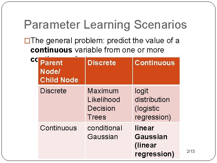
Parameter Learning Scenarios �The general problem: predict the value of a continuous variable from one or more continuous features. Parent Discrete Continuous Node/ Child Node Discrete Continuous Maximum Likelihood Decision Trees logit distribution (logistic regression) conditional Gaussian linear Gaussian (linear regression) 2/13

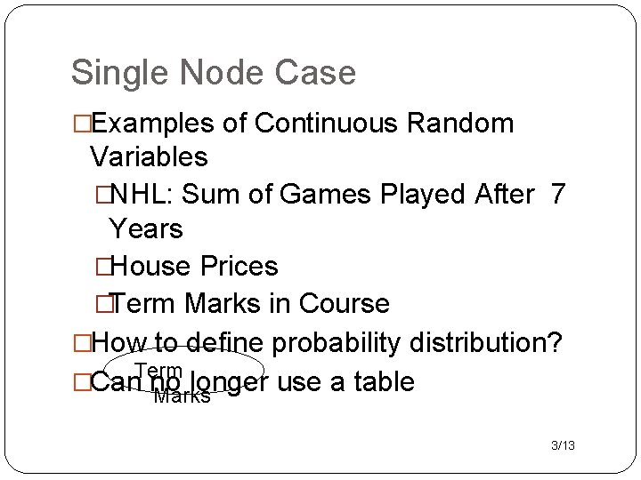
Single Node Case �Examples of Continuous Random Variables �NHL: Sum of Games Played After 7 Years �House Prices �Term Marks in Course �How to define probability distribution? Term �Can no longer use a table Marks 3/13

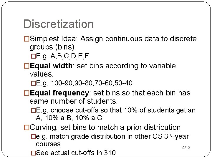
Discretization �Simplest Idea: Assign continuous data to discrete groups (bins). �E. g. A, B, C, D, E, F �Equal width: set bins according to variable values. �E. g. 100 -90, 90 -80, 70 -60, 50 -40 �Equal frequency: set bins so that each bin has same number of students. �E. g. choose cut-offs so that 10% of students get an A, 10% a B, 10% a C �Curving: set bins to match a prior distribution �e. g. match grade distribution in other CS 3 rd-year courses �See actual cut-offs in 310 4/13

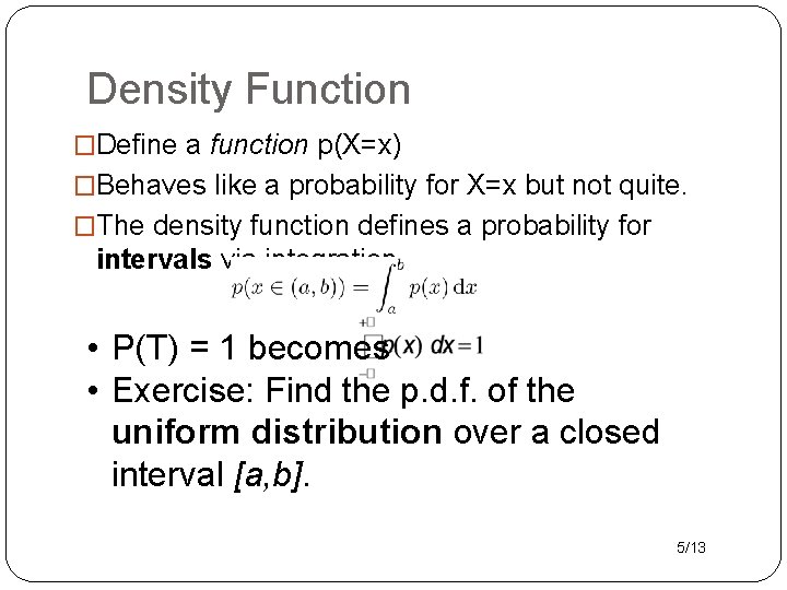
Density Function �Define a function p(X=x) �Behaves like a probability for X=x but not quite. �The density function defines a probability for intervals via integration. • P(T) = 1 becomes • Exercise: Find the p. d. f. of the uniform distribution over a closed interval [a, b]. 5/13

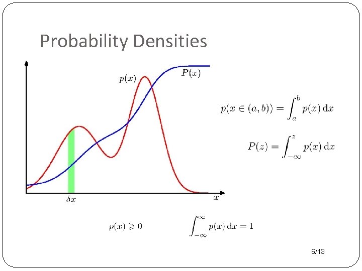
Probability Densities 6/13

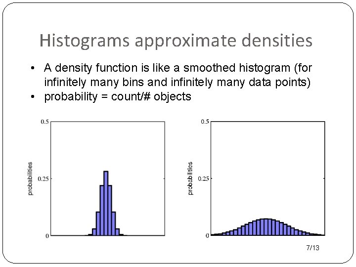
Histograms approximate densities • A density function is like a smoothed histogram (for infinitely many bins and infinitely many data points) • probability = count/# objects 7/13

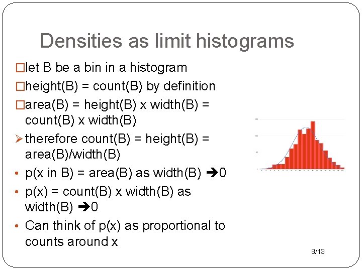
Densities as limit histograms �let B be a bin in a histogram �height(B) = count(B) by definition �area(B) = height(B) x width(B) = count(B) x width(B) Ø therefore count(B) = height(B) = area(B)/width(B) • p(x in B) = area(B) as width(B) 0 • p(x) = count(B) x width(B) as width(B) 0 • Can think of p(x) as proportional to counts around x 8/13

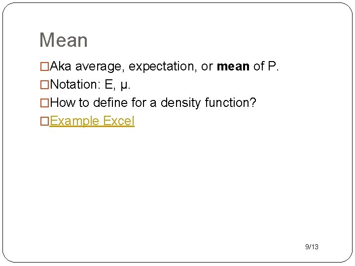
Mean �Aka average, expectation, or mean of P. �Notation: E, µ. �How to define for a density function? �Example Excel 9/13

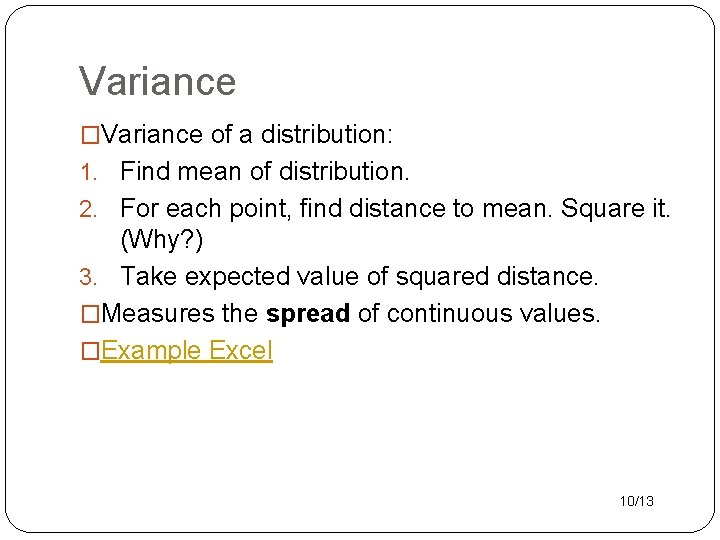
Variance �Variance of a distribution: 1. Find mean of distribution. 2. For each point, find distance to mean. Square it. (Why? ) 3. Take expected value of squared distance. �Measures the spread of continuous values. �Example Excel 10/13

The Gaussian Density Function

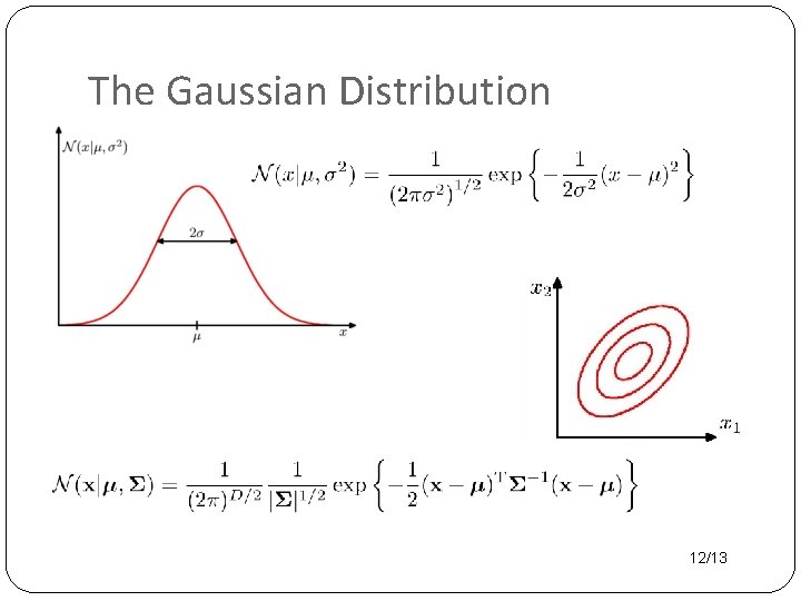
The Gaussian Distribution 12/13

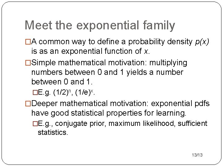
Meet the exponential family �A common way to define a probability density p(x) is as an exponential function of x. �Simple mathematical motivation: multiplying numbers between 0 and 1 yields a number between 0 and 1. �E. g. (1/2)n, (1/e)x. �Deeper mathematical motivation: exponential pdfs have good statistical properties for learning. �E. g. , conjugate prior, maximum likelihood, sufficient statistics. 13/13

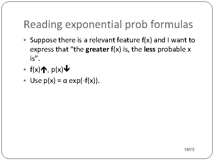
Reading exponential prob formulas • Suppose there is a relevant feature f(x) and I want to express that “the greater f(x) is, the less probable x is”. • f(x) , p(x) • Use p(x) = α exp(-f(x)). 14/13

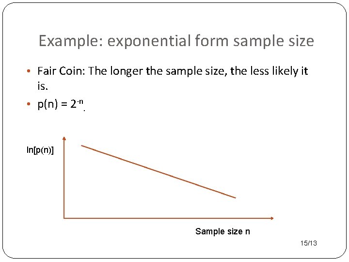
Example: exponential form sample size • Fair Coin: The longer the sample size, the less likely it is. • p(n) = 2 -n. ln[p(n)] Sample size n 15/13

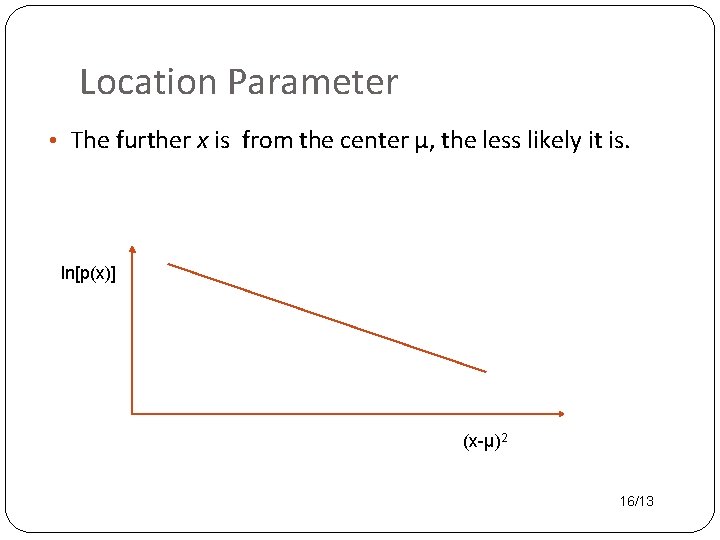
Location Parameter • The further x is from the center μ, the less likely it is. ln[p(x)] (x-μ)2 16/13

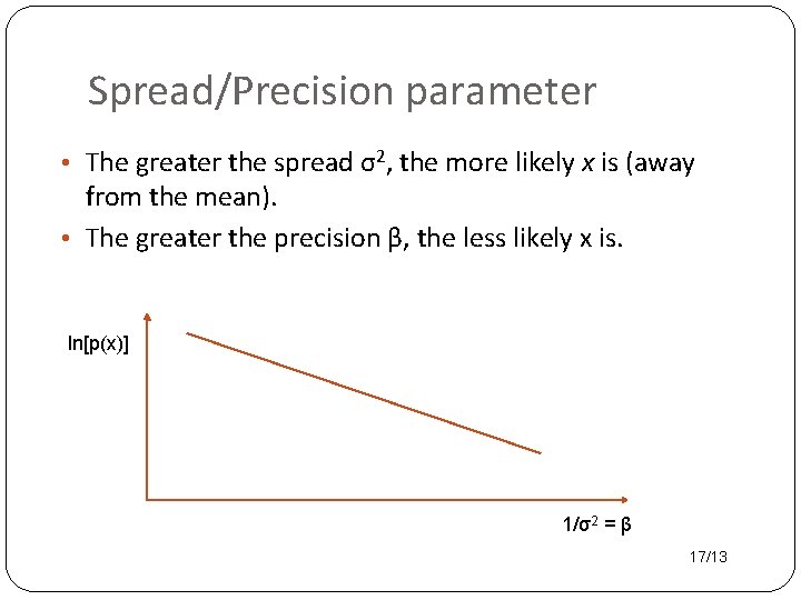
Spread/Precision parameter • The greater the spread σ2, the more likely x is (away from the mean). • The greater the precision β, the less likely x is. ln[p(x)] 1/σ2 = β 17/13

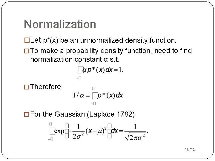
Normalization �Let p*(x) be an unnormalized density function. � To make a probability density function, need to find normalization constant α s. t. � Therefore � For the Gaussian (Laplace 1782) 18/13

Maximum Likelihood Learning �Same fundamental idea as with discrete variables: maximize data likelihood given parameters. �The likelihood function for Gausssian distribution: �Log-likelihood function �Find derivatives of L, set to 0. �For details see text and assignment. �Results: �For mean, the MLE estimate is the sample mean �For standard deviation the MLE estimate is the sample sd Ø MLE estimates track the data 21/13

Parameter Learning: Discrete Parents

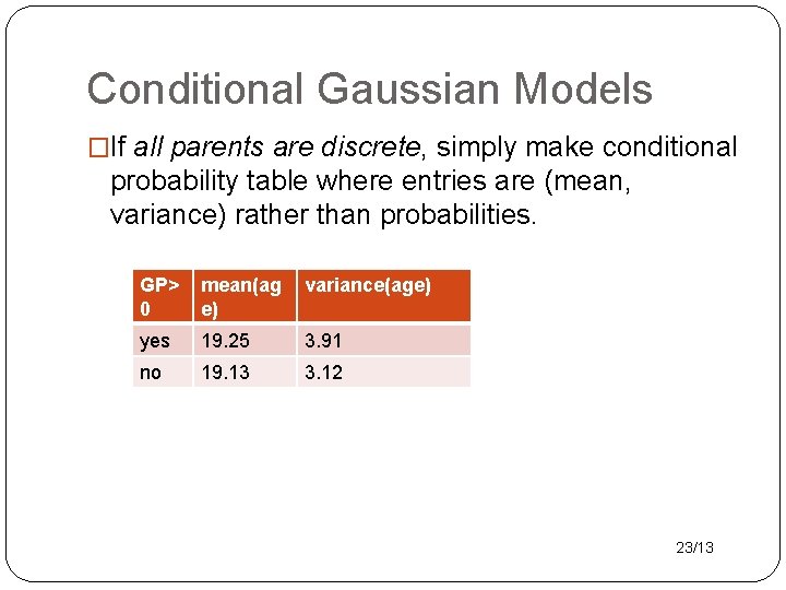
Conditional Gaussian Models �If all parents are discrete, simply make conditional probability table where entries are (mean, variance) rather than probabilities. GP> 0 mean(ag e) variance(age) yes 19. 25 3. 91 no 19. 13 3. 12 23/13

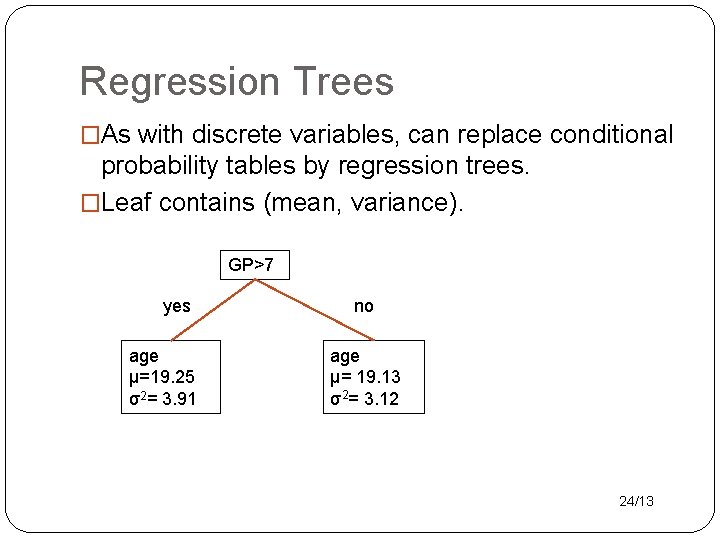
Regression Trees �As with discrete variables, can replace conditional probability tables by regression trees. �Leaf contains (mean, variance). GP>7 yes age μ=19. 25 σ2= 3. 91 no age μ= 19. 13 σ2= 3. 12 24/13

Covariance and Correlation Single continuous parent

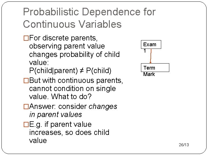
Probabilistic Dependence for Continuous Variables �For discrete parents, observing parent value changes probability of child value: P(child|parent) ≠ P(child) �But with continuous parents, cannot condition on single value. What to do? �Answer: consider changes in parent values �E. g. if parent value increases, so does child value Exam 1 Term Mark 26/13

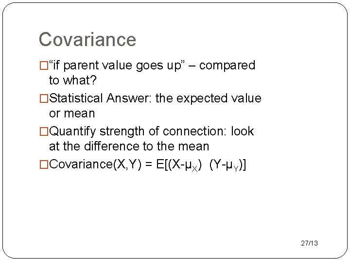
Covariance �“if parent value goes up” – compared to what? �Statistical Answer: the expected value or mean �Quantify strength of connection: look at the difference to the mean �Covariance(X, Y) = E[(X-μX) (Y-μY)] 27/13

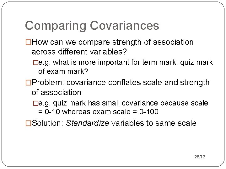
Comparing Covariances �How can we compare strength of association across different variables? �e. g. what is more important for term mark: quiz mark of exam mark? �Problem: covariance conflates scale and strength of association �e. g. quiz mark has small covariance because scale = 0 -10 whereas exam scale = 0 -100 �Solution: Standardize variables to same scale 28/13

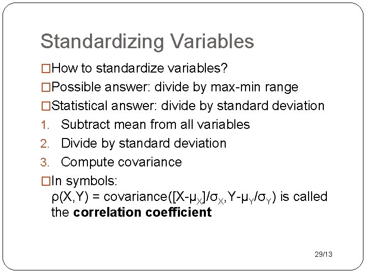
Standardizing Variables �How to standardize variables? �Possible answer: divide by max-min range �Statistical answer: divide by standard deviation 1. Subtract mean from all variables 2. Divide by standard deviation 3. Compute covariance �In symbols: ρ(X, Y) = covariance([X-μX]/σX, Y-μY/σY) is called the correlation coefficient 29/13

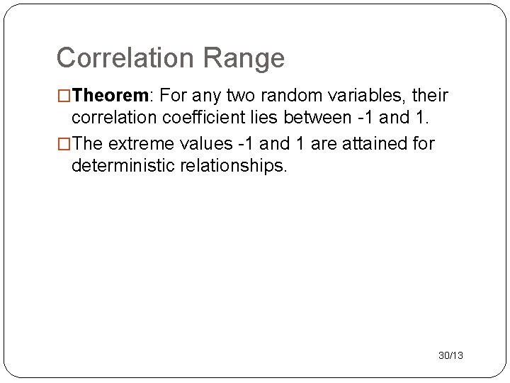
Correlation Range �Theorem: For any two random variables, their correlation coefficient lies between -1 and 1. �The extreme values -1 and 1 are attained for deterministic relationships. 30/13

Predictive Modelling

Predictive Relationship �Correlation tells us that the probability of the child node varies with the parent nodes. �But that does not define a conditional probability P(child node value|parent node value). �Strategy: 1. Build model to predict a child node value given parent node values. 2. Incorporate (Gaussian) uncertainty to turn prediction into probability. 32/13

Linear Regression

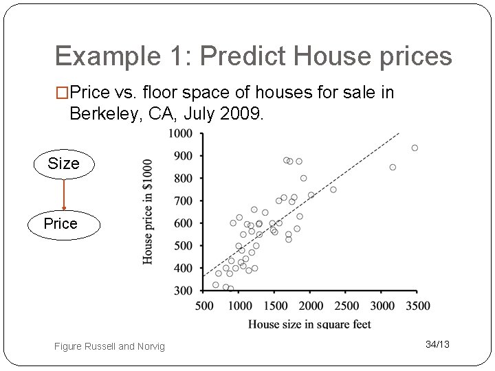
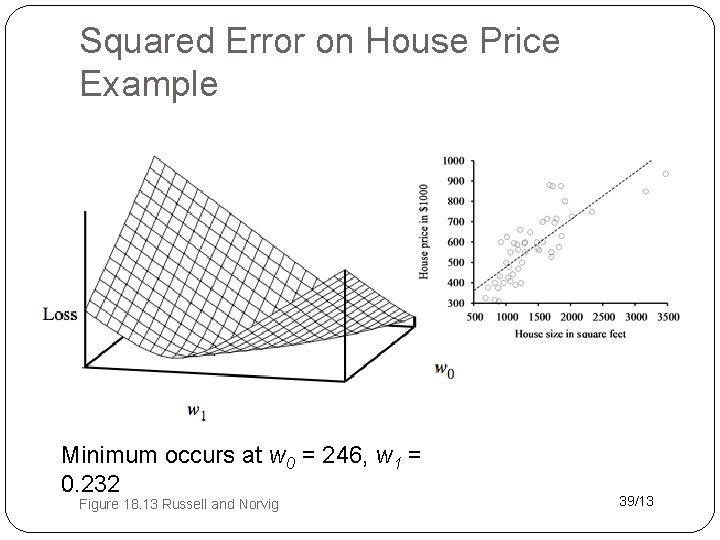
Example 1: Predict House prices �Price vs. floor space of houses for sale in Berkeley, CA, July 2009. Size Price Figure Russell and Norvig 34/13

Grading Example • Predict: final percentage mark for student. • Features: assignment grades, midterm exam, final exam. • Questions for linear regression: • I forgot the weights of components. Can you recover them from a spreadsheet of the final grades? • How important is each component, actually? Could I guess well someone’s final mark given their assignments? Given their exams? 35/13

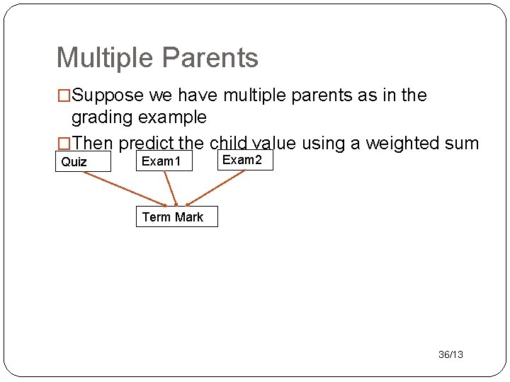
Multiple Parents �Suppose we have multiple parents as in the grading example �Then predict the child value using a weighted sum Quiz Exam 1 Exam 2 Term Mark 36/13

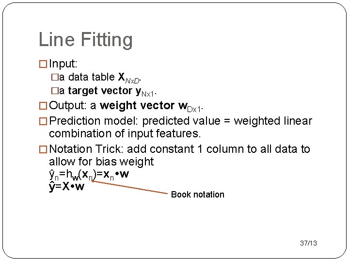
Line Fitting � Input: �a data table XNx. D. �a target vector y. Nx 1. � Output: a weight vector w. Dx 1. � Prediction model: predicted value = weighted linear combination of input features. � Notation Trick: add constant 1 column to all data to allow for bias weight ŷn=hw(xn)=xn w ŷ=X w Book notation 37/13

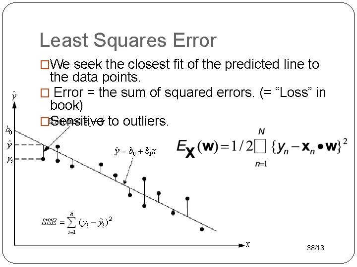
Least Squares Error �We seek the closest fit of the predicted line to the data points. � Error = the sum of squared errors. (= “Loss” in book) �Sensitive to outliers. 38/13

Squared Error on House Price Example Minimum occurs at w 0 = 246, w 1 = 0. 232 Figure 18. 13 Russell and Norvig 39/13

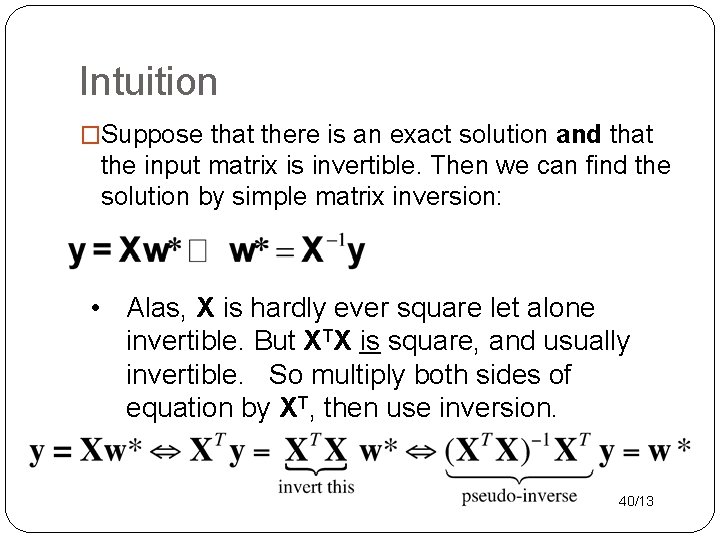
Intuition �Suppose that there is an exact solution and that the input matrix is invertible. Then we can find the solution by simple matrix inversion: • Alas, X is hardly ever square let alone invertible. But XTX is square, and usually invertible. So multiply both sides of equation by XT, then use inversion. 40/13

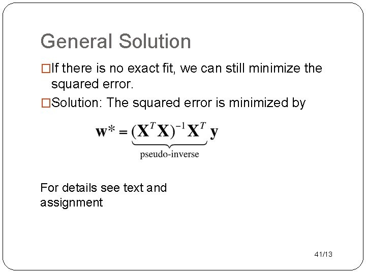
General Solution �If there is no exact fit, we can still minimize the squared error. �Solution: The squared error is minimized by For details see text and assignment 41/13

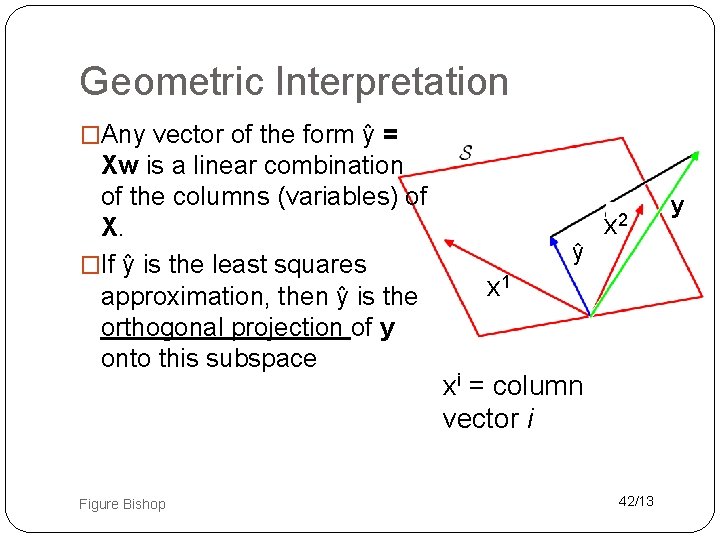
Geometric Interpretation �Any vector of the form ŷ = Xw is a linear combination of the columns (variables) of X. �If ŷ is the least squares approximation, then ŷ is the orthogonal projection of y onto this subspace Figure Bishop ŷ x 2 x 1 xi = column vector i 42/13 y

Probabilistic Model Prediction + Uncertainty = Probability

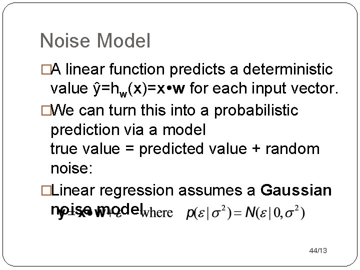
Noise Model �A linear function predicts a deterministic value ŷ=hw(x)=x w for each input vector. �We can turn this into a probabilistic prediction via a model true value = predicted value + random noise: �Linear regression assumes a Gaussian noise model 44/13

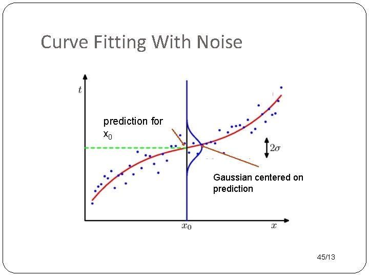
Curve Fitting With Noise prediction for x 0 Gaussian centered on prediction 45/13

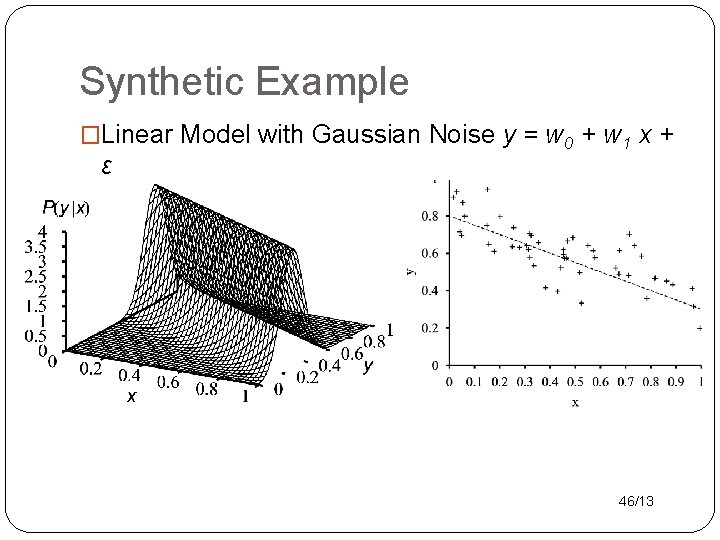
Synthetic Example �Linear Model with Gaussian Noise y = w 0 + w 1 x + ε 46/13

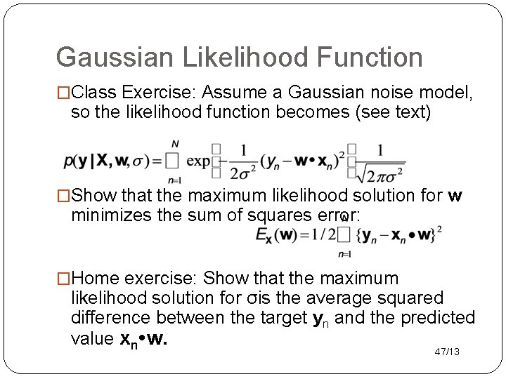
Gaussian Likelihood Function �Class Exercise: Assume a Gaussian noise model, so the likelihood function becomes (see text) �Show that the maximum likelihood solution for w minimizes the sum of squares error: �Home exercise: Show that the maximum likelihood solution for σis the average squared difference between the target yn and the predicted value xn w. 47/13

Mixed/Hybrid Parents The General Case

Hybrid Parents �Parents could contain both continuous and discrete data �One option: use regression tree �Another option: treat discrete variables as if they were continuous. 1. turn all discrete variables into binary (Boolean variables) (dummy variables, one-of-k coding, one-hot vector) 2. Use the fact that 1 and 0 behave like T and F (kind of). 49/13

Overfitting 50/13

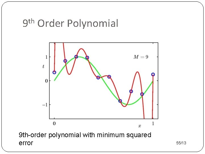
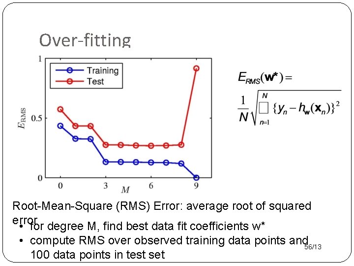
Overfitting �Maximum likelihood treats data sample as if it represents complete information. �For both discrete BNs and regression models �For small samples, this leads to extreme results. �For regression models, we get overfitting: test set performance is much worse than training set. �A deeper perspective on overfitting is the bias- variance trade-off to be discussed later. 51/13

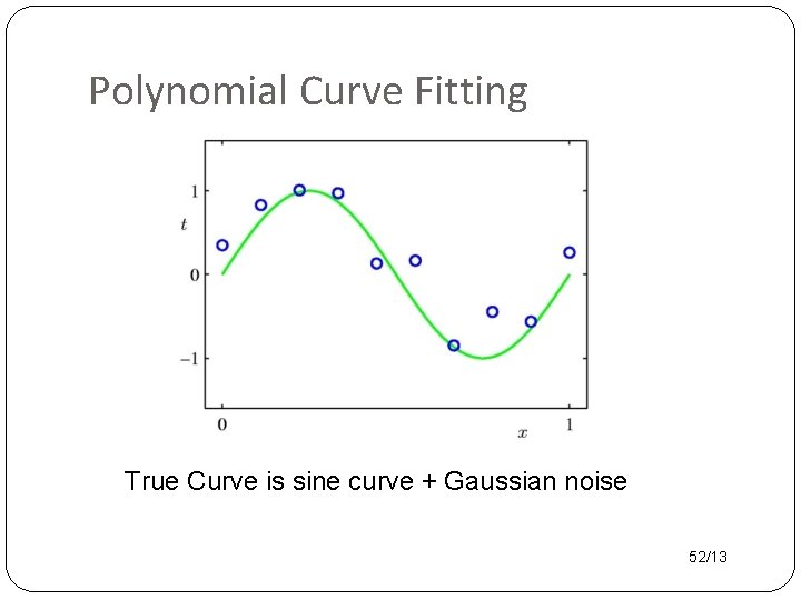
Polynomial Curve Fitting True Curve is sine curve + Gaussian noise 52/13

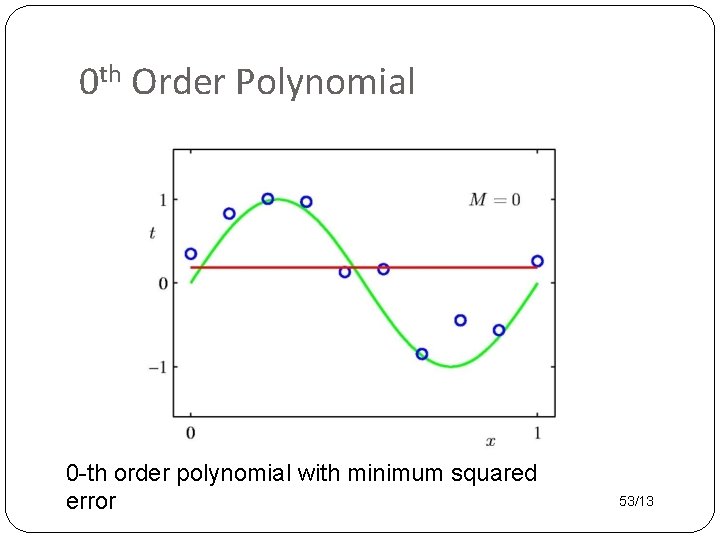
0 th Order Polynomial 0 -th order polynomial with minimum squared error 53/13

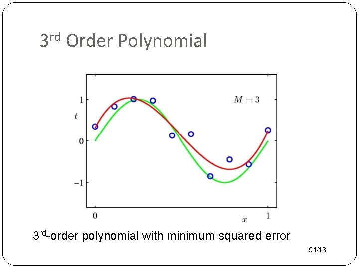
3 rd Order Polynomial 3 rd-order polynomial with minimum squared error 54/13

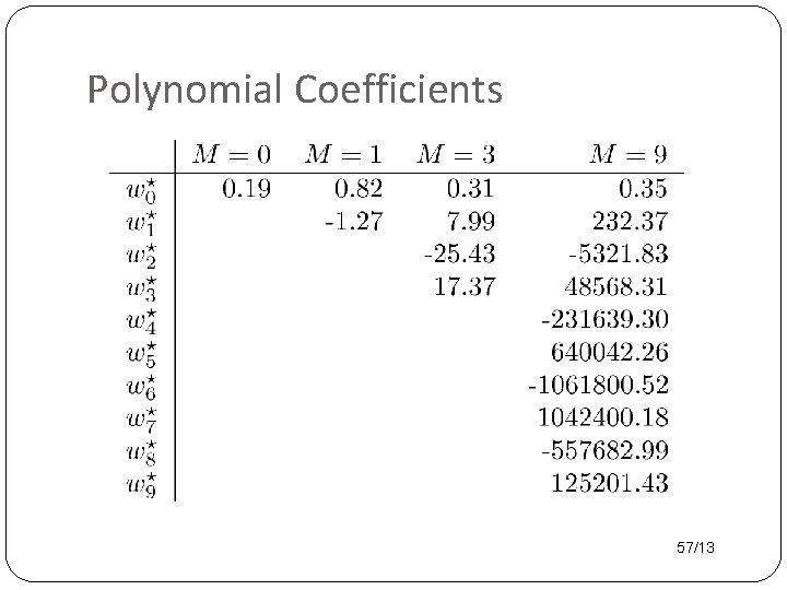
9 th Order Polynomial 9 th-order polynomial with minimum squared error 55/13

Over-fitting Root-Mean-Square (RMS) Error: average root of squared error • for degree M, find best data fit coefficients w* • compute RMS over observed training data points and 56/13 100 data points in test set

Polynomial Coefficients 57/13

Regularization

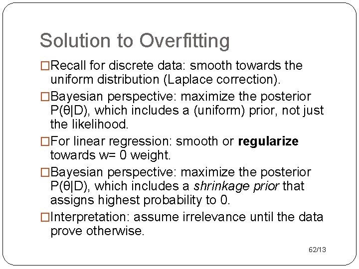
Solution to Overfitting �Recall for discrete data: smooth towards the uniform distribution (Laplace correction). �Bayesian perspective: maximize the posterior P(θ|D), which includes a (uniform) prior, not just the likelihood. �For linear regression: smooth or regularize towards w= 0 weight. �Bayesian perspective: maximize the posterior P(θ|D), which includes a shrinkage prior that assigns highest probability to 0. �Interpretation: assume irrelevance until the data prove otherwise. 62/13

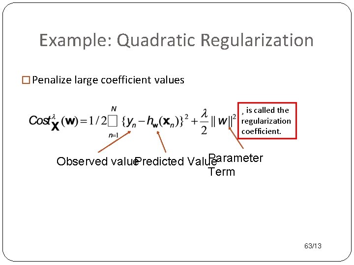
Example: Quadratic Regularization � Penalize large coefficient values ¸ is called the regularization coefficient. Parameter Observed value. Predicted Value Term 63/13

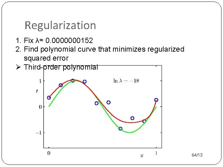
Regularization 1. Fix λ≈ 0. 0000000152 2. Find polynomial curve that minimizes regularized squared error Ø Third-order polynomial 64/13

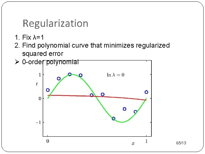
Regularization 1. Fix λ=1 2. Find polynomial curve that minimizes regularized squared error Ø 0 -order polynomial 65/13

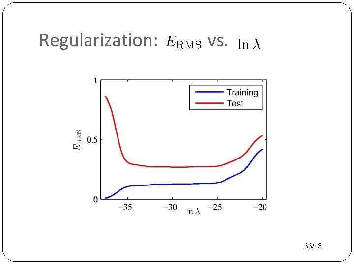
Regularization: vs. 66/13

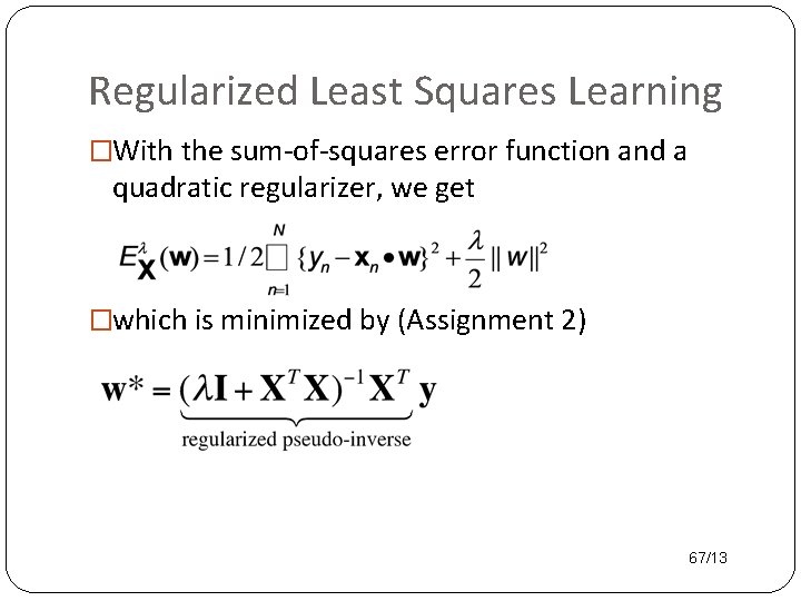
Regularized Least Squares Learning �With the sum-of-squares error function and a quadratic regularizer, we get �which is minimized by (Assignment 2) 67/13

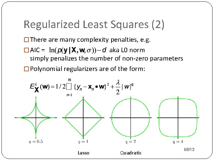
Regularized Least Squares (2) � There are many complexity penalties, e. g. � AIC = aka L 0 norm simply penalizes the number of non-zero parameters � Polynomial regularizers are of the form: Lasso Quadratic 68/13

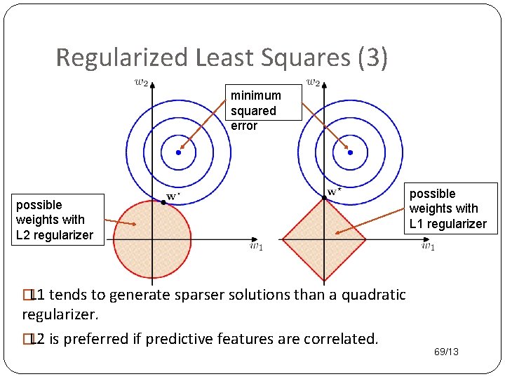
Regularized Least Squares (3) minimum squared error possible weights with L 2 regularizer possible weights with L 1 regularizer �L 1 tends to generate sparser solutions than a quadratic regularizer. �L 2 is preferred if predictive features are correlated. 69/13

Standardization �If the predictive features are on different scales, a single regularization coefficient λ is not adequate. �e. g. �Solution: Standardize variables before choosing λ. 70/13

Evaluating Models and Parameters By Cross-Validation 71/13

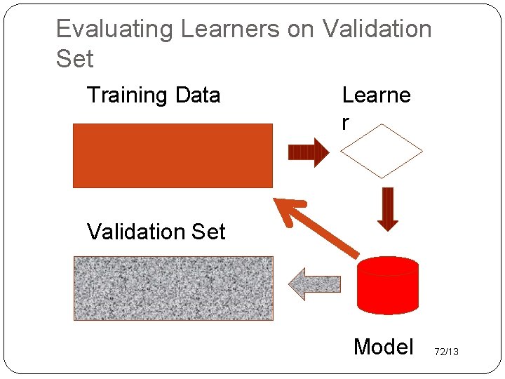
Evaluating Learners on Validation Set Training Data Learne r Validation Set Model 72/13

What if there is no validation set? �What does training error tell me about the generalization performance on a hypothetical validation set? �Scenario 1: You run a big pharmaceutical company. Your new drug looks pretty good on the trials you’ve done so far. The government tells you to test it on another 10, 000 patients. �Scenario 2: Your friendly machine learning instructor provides you with another validation set. 73/13 �What if you can’t get more validation data?

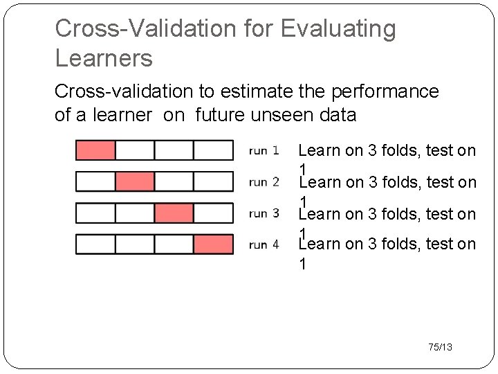
Cross-Validation for Evaluating Learners Cross-validation to estimate the performance of a learner on future unseen data Learn on 3 folds, test on 1 75/13

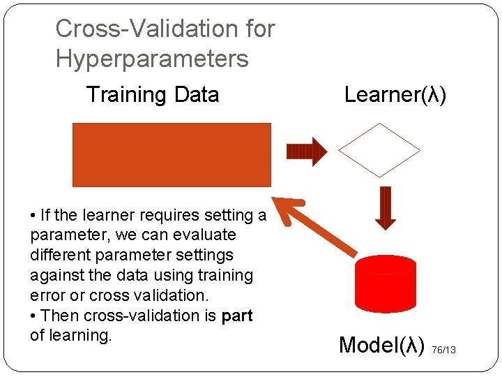
Cross-Validation for Hyperparameters Training Data • If the learner requires setting a parameter, we can evaluate different parameter settings against the data using training error or cross validation. • Then cross-validation is part of learning. Learner(λ) Model(λ) 76/13

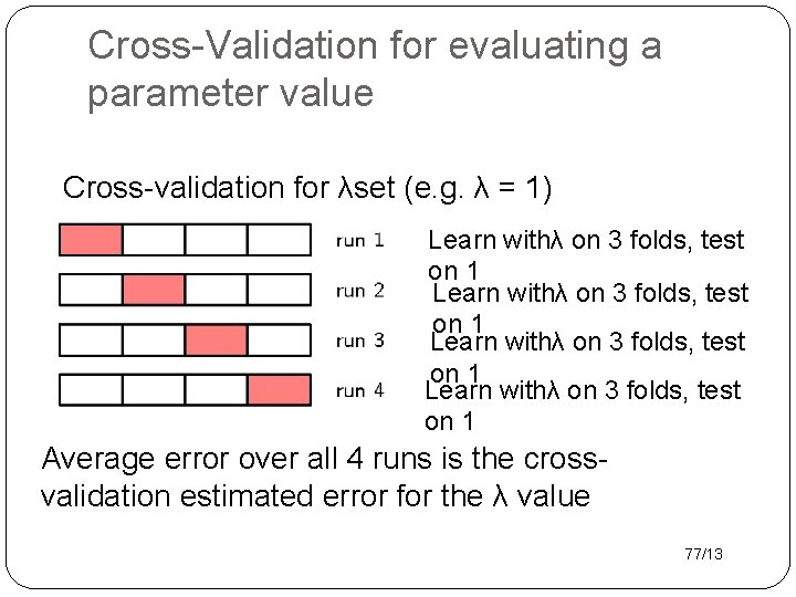
Cross-Validation for evaluating a parameter value Cross-validation for λset (e. g. λ = 1) Learn withλ on 3 folds, test on 1 Average error over all 4 runs is the crossvalidation estimated error for the λ value 77/13

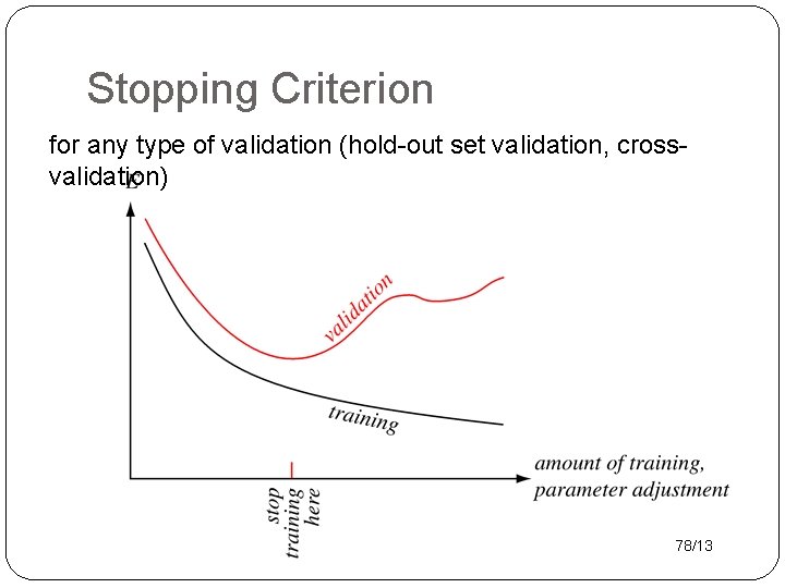
Stopping Criterion for any type of validation (hold-out set validation, crossvalidation) 78/13

Regression With Basis Functions Details in Assignment

Nonlinear Features �We can increase the power of linear regression by using functions of the input features instead of the input features. �Like sufficient statistics, but called basis functions in the context of regression �Linear regression can then be used to assign weights to the basis functions. �We will see several examples (Assignment 2) �Neural nets are a way to learn powerful basis functions 80/13

Conclusion �Density functions define probabilities for continuous random variables �The Gaussian density function is the most prominent. �There is a typical value called the mean �probability(x) decreases with distance from x �Linear regression predicts a continuous value given a set of continuous input features using a linear model ŷ=x w �Uncertainty in prediction is modelled as a Gaussian centered on the prediction ŷ � Can combine linear regression with nonlinear basis functions φ(x) 81/13