Linear regression models Simple Linear Regression History Developed

Linear regression models

Simple Linear Regression

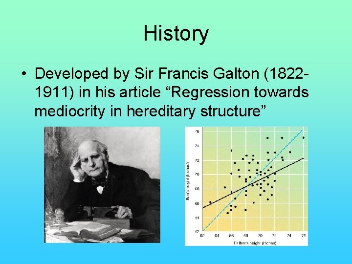
History • Developed by Sir Francis Galton (18221911) in his article “Regression towards mediocrity in hereditary structure”

Purposes: • To describe the linear relationship between two continuous variables, the response variable (yaxis) and a single predictor variable (x-axis) • To determine how much of the variation in Y can be explained by the linear relationship with X and how much of this relationship remains unexplained • To predict new values of Y from new values of X

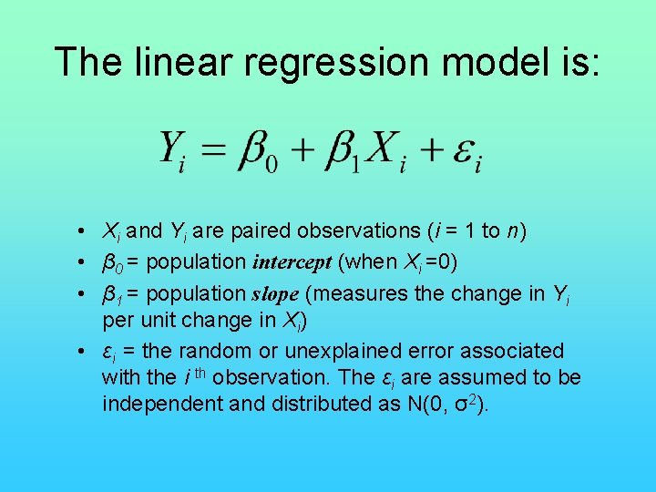
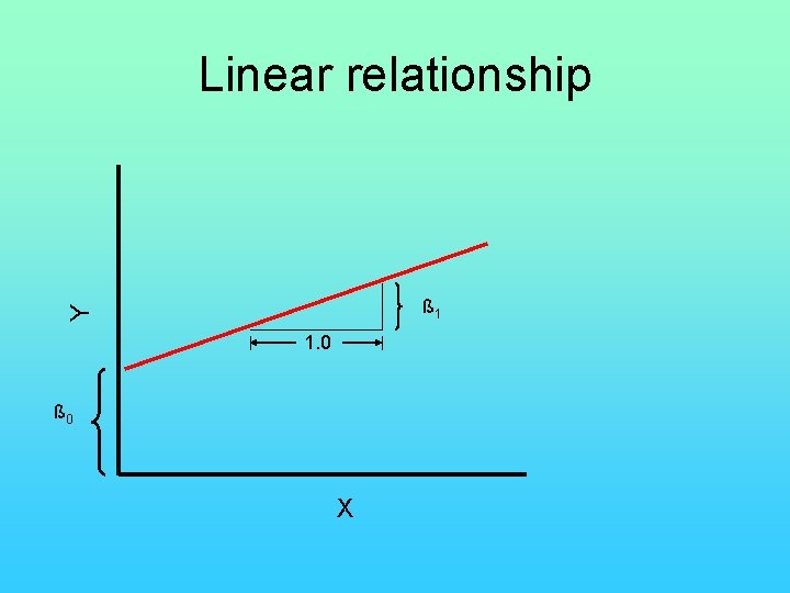
The linear regression model is: • Xi and Yi are paired observations (i = 1 to n) • β 0 = population intercept (when Xi =0) • β 1 = population slope (measures the change in Yi per unit change in Xi) • εi = the random or unexplained error associated with the i th observation. The εi are assumed to be independent and distributed as N(0, σ2).

Linear relationship Y ß 1 1. 0 ß 0 X

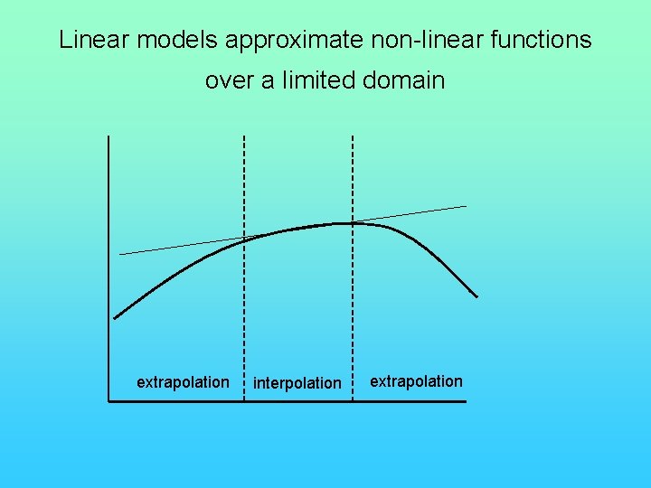
Linear models approximate non-linear functions over a limited domain extrapolation interpolation extrapolation

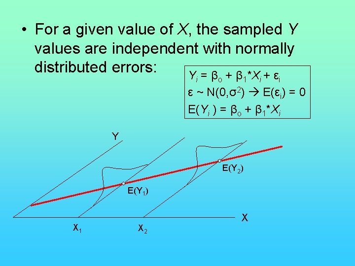
• For a given value of X, the sampled Y values are independent with normally distributed errors: Y = β + β *X + ε i o 1 i i ε ~ N(0, σ2) E(εi) = 0 E(Yi ) = βo + β 1*Xi Y E(Y 2) E(Y 1) X 1 X X 2

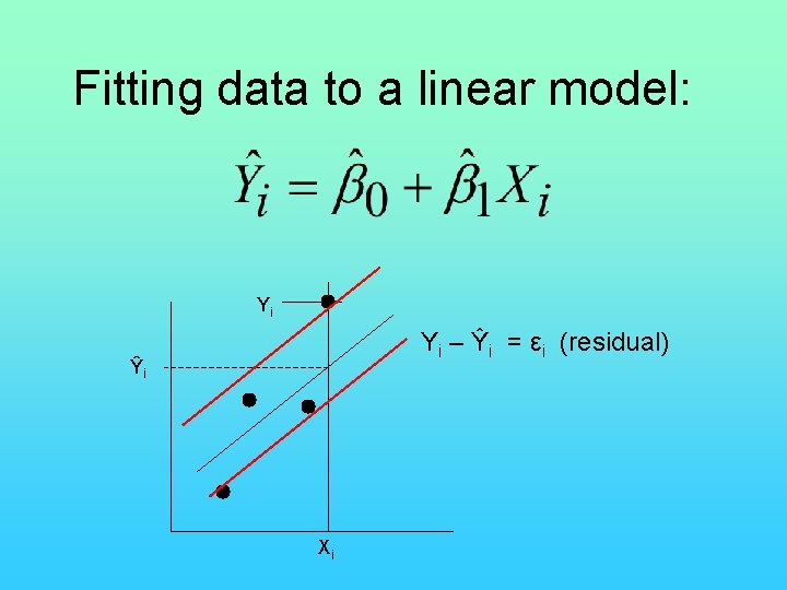
Fitting data to a linear model: Yi Yi – Ŷi = εi (residual) Ŷi Xi

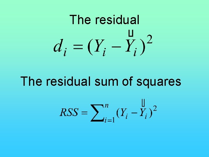
The residual sum of squares

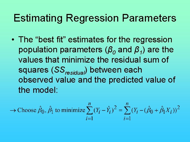
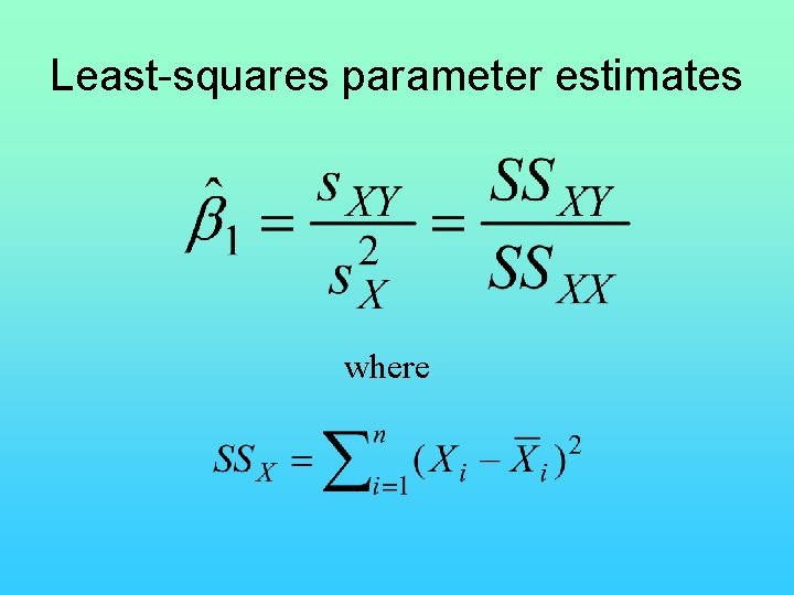
Estimating Regression Parameters • The “best fit” estimates for the regression population parameters (β 0 and β 1) are the values that minimize the residual sum of squares (SSresidual) between each observed value and the predicted value of the model:

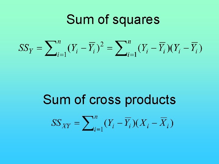
Sum of squares Sum of cross products

Least-squares parameter estimates where

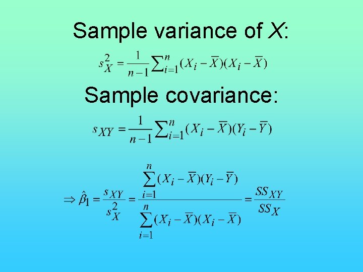
Sample variance of X: Sample covariance:

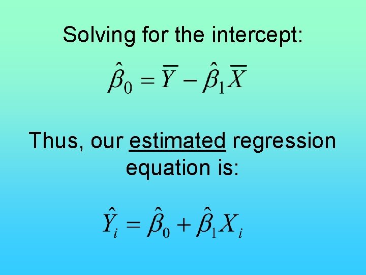
Solving for the intercept: Thus, our estimated regression equation is:

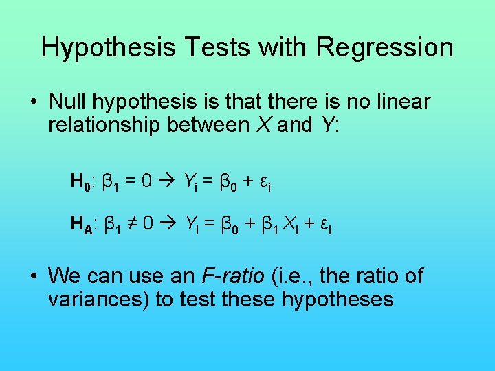
Hypothesis Tests with Regression • Null hypothesis is that there is no linear relationship between X and Y: H 0: β 1 = 0 Y i = β 0 + ε i H A: β 1 ≠ 0 Y i = β 0 + β 1 X i + ε i • We can use an F-ratio (i. e. , the ratio of variances) to test these hypotheses

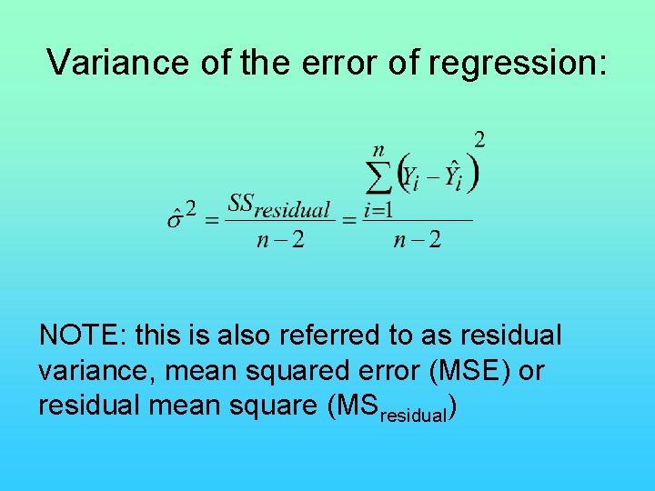
Variance of the error of regression: NOTE: this is also referred to as residual variance, mean squared error (MSE) or residual mean square (MSresidual)

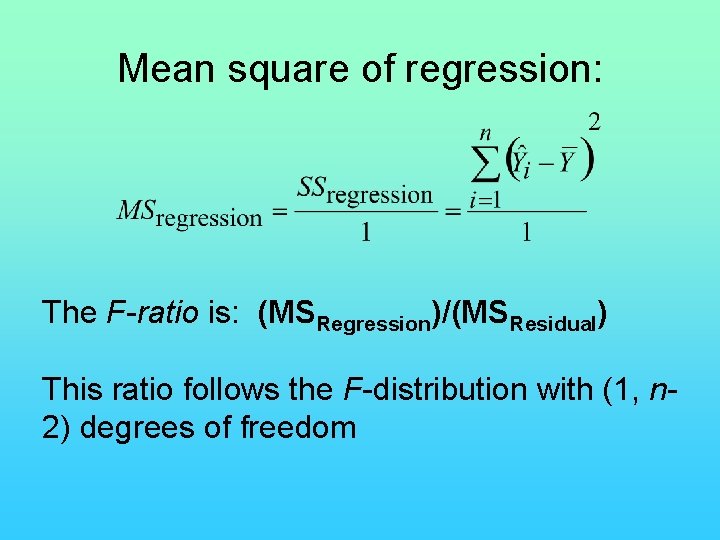
Mean square of regression: The F-ratio is: (MSRegression)/(MSResidual) This ratio follows the F-distribution with (1, n 2) degrees of freedom

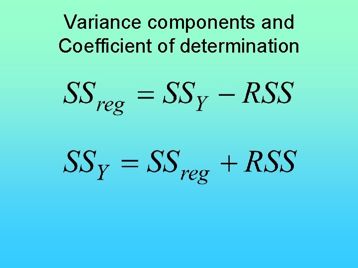
Variance components and Coefficient of determination

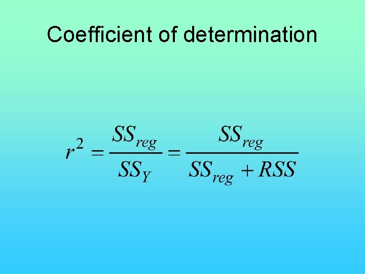
Coefficient of determination

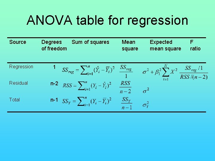
ANOVA table for regression Source Regression Degrees Sum of squares of freedom 1 Residual n-2 Total n-1 Mean square Expected mean square F ratio

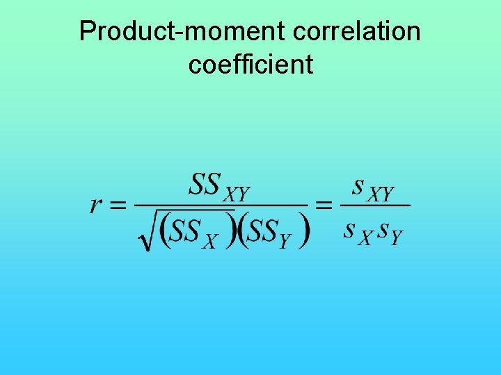
Product-moment correlation coefficient

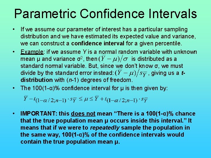
Parametric Confidence Intervals • If we assume our parameter of interest has a particular sampling distribution and we have estimated its expected value and variance, we can construct a confidence interval for a given percentile. • Example: if we assume Y is a normal random variable with unknown mean μ and variance σ2, then is distributed as a standard normal variable. But, since we don’t know σ, we must divide by the standard error instead: , giving us a tdistribution with (n-1) degrees of freedom. • The 100(1 -α)% confidence interval for μ is then given by: • IMPORTANT: this does not mean “There is a 100(1 -α)% chance that the true population mean μ occurs inside this interval. ” It means that if we were to repeatedly sample the population in the same way, 100(1 -α)% of the confidence intervals would contain the true population mean μ.

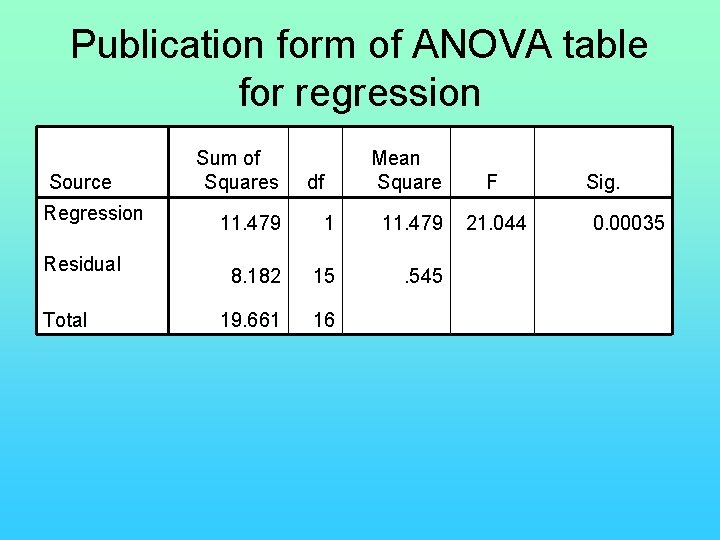
Publication form of ANOVA table for regression Source Regression Residual Total Sum of Squares df Mean Square F 21. 044 11. 479 1 11. 479 8. 182 15 . 545 19. 661 16 Sig. 0. 00035

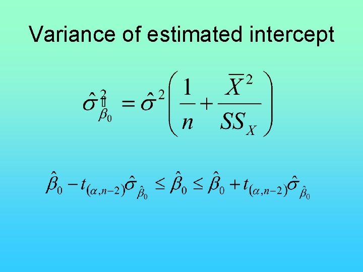
Variance of estimated intercept

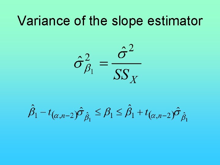
Variance of the slope estimator

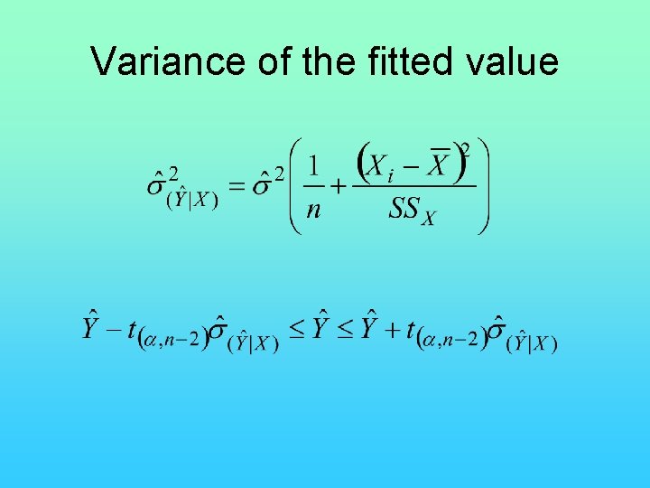
Variance of the fitted value

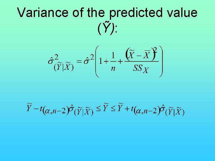
Variance of the predicted value (Ỹ):

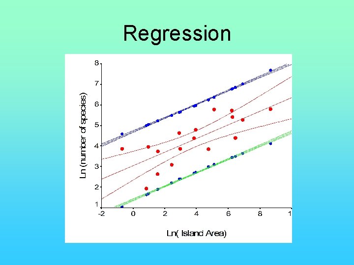
Regression

Assumptions of regression • The linear model correctly describes the functional relationship between X and Y • The X variable is measured without error • For a given value of X, the sampled Y values are independent with normally distributed errors • Variances are constant along the regression line

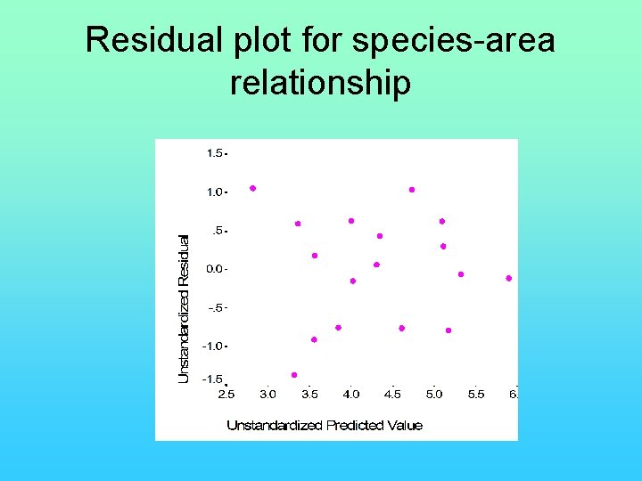
Residual plot for species-area relationship