Linear Regression Dr A Emamzadeh 1 662021 What

Linear Regression Dr. A. Emamzadeh 1 6/6/2021

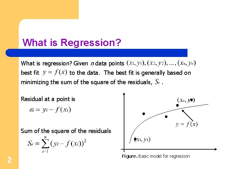
What is Regression? What is regression? Given n data points best fit to the data. The best fit is generally based on minimizing the sum of the square of the residuals, . Residual at a point is Sum of the square of the residuals 2 Figure. Basic model for regression

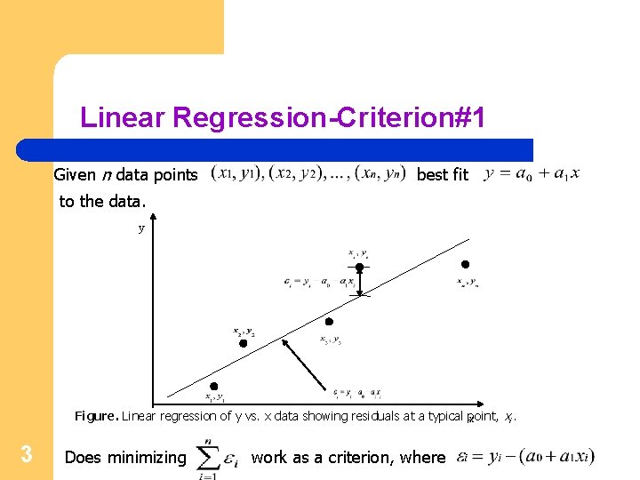
Linear Regression-Criterion#1 Given n data points best fit to the data. y Figure. Linear regression of y vs. x data showing residuals at a typical point, xi. x 3 Does minimizing work as a criterion, where

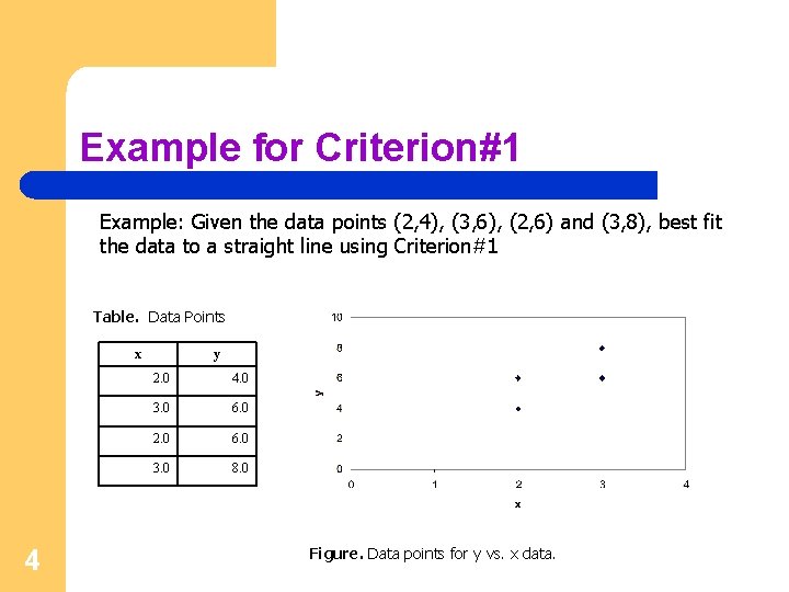
Example for Criterion#1 Example: Given the data points (2, 4), (3, 6), (2, 6) and (3, 8), best fit the data to a straight line using Criterion#1 Table. Data Points x 4 y 2. 0 4. 0 3. 0 6. 0 2. 0 6. 0 3. 0 8. 0 Figure. Data points for y vs. x data.

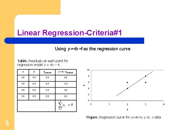
Linear Regression-Criteria#1 Using y=4 x-4 as the regression curve Table. Residuals at each point for regression model y = 4 x – 4. x y ypredicted ε = y - ypredicted 2. 0 4. 0 0. 0 3. 0 6. 0 8. 0 -2. 0 6. 0 4. 0 2. 0 3. 0 8. 0 0. 0 Figure. Regression curve for y=4 x-4, y vs. x data 5

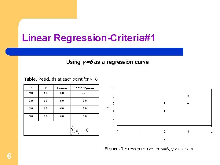
Linear Regression-Criteria#1 Using y=6 as a regression curve Table. Residuals at each point for y=6 x y ypredicted ε = y - ypredicted 2. 0 4. 0 6. 0 -2. 0 3. 0 6. 0 0. 0 2. 0 6. 0 0. 0 3. 0 8. 0 6. 0 2. 0 Figure. Regression curve for y=6, y vs. x data 6

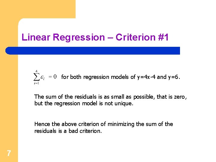
Linear Regression – Criterion #1 for both regression models of y=4 x-4 and y=6. The sum of the residuals is as small as possible, that is zero, but the regression model is not unique. Hence the above criterion of minimizing the sum of the residuals is a bad criterion. 7

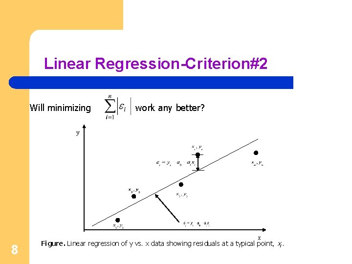
Linear Regression-Criterion#2 Will minimizing work any better? y x 8 Figure. Linear regression of y vs. x data showing residuals at a typical point, xi.

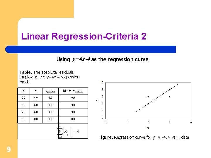
Linear Regression-Criteria 2 Using y=4 x-4 as the regression curve Table. The absolute residuals employing the y=4 x-4 regression model x y ypredicted |ε| = |y - ypredicted| 2. 0 4. 0 0. 0 3. 0 6. 0 8. 0 2. 0 6. 0 4. 0 2. 0 3. 0 8. 0 0. 0 Figure. Regression curve for y=4 x-4, y vs. x data 9

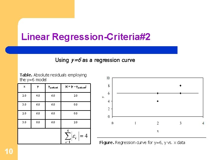
Linear Regression-Criteria#2 Using y=6 as a regression curve Table. Absolute residuals employing the y=6 model x y ypredicted |ε| = |y – ypredicted| 2. 0 4. 0 6. 0 2. 0 3. 0 6. 0 0. 0 2. 0 6. 0 0. 0 3. 0 8. 0 6. 0 2. 0 Figure. Regression curve for y=6, y vs. x data 10

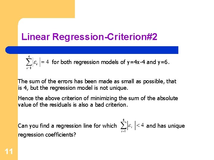
Linear Regression-Criterion#2 for both regression models of y=4 x-4 and y=6. The sum of the errors has been made as small as possible, that is 4, but the regression model is not unique. Hence the above criterion of minimizing the sum of the absolute value of the residuals is also a bad criterion. Can you find a regression line for which regression coefficients? 11 and has unique

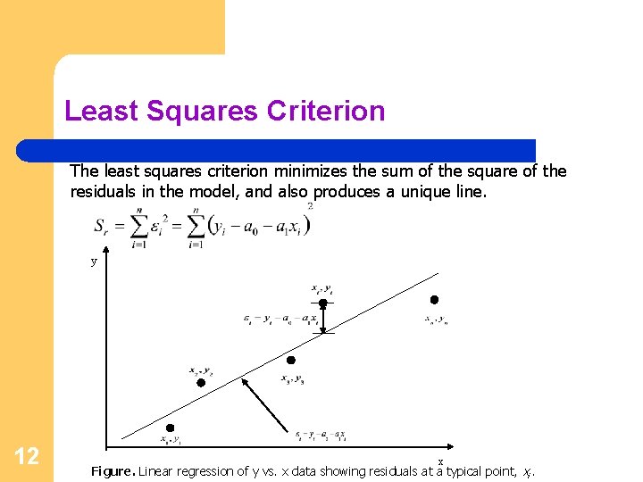
Least Squares Criterion The least squares criterion minimizes the sum of the square of the residuals in the model, and also produces a unique line. y 12 x Figure. Linear regression of y vs. x data showing residuals at a typical point, xi.

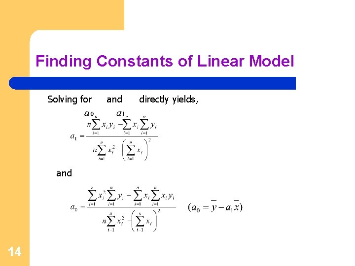
Finding Constants of Linear Model Minimize the sum of the square of the residuals: To find giving 13 and we minimize with respect to and .

Finding Constants of Linear Model Solving for and 14 and directly yields,

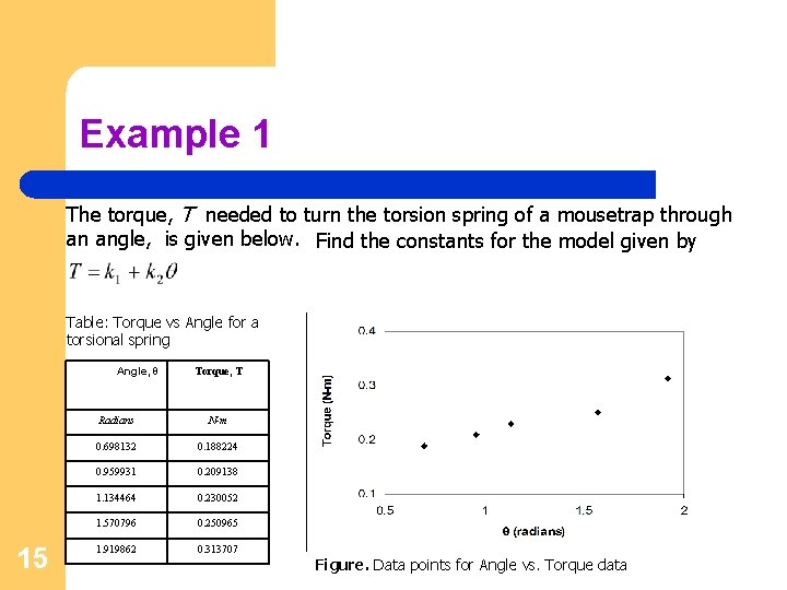
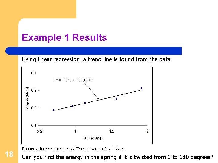
Example 1 The torque, T needed to turn the torsion spring of a mousetrap through an angle, is given below. Find the constants for the model given by Table: Torque vs Angle for a torsional spring Angle, θ 15 Torque, T Radians N-m 0. 698132 0. 188224 0. 959931 0. 209138 1. 134464 0. 230052 1. 570796 0. 250965 1. 919862 0. 313707 Figure. Data points for Angle vs. Torque data

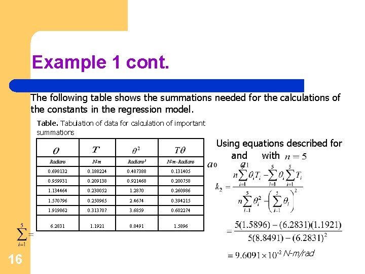
Example 1 cont. The following table shows the summations needed for the calculations of the constants in the regression model. Table. Tabulation of data for calculation of important summations 16 Radians N-m Radians 2 N-m-Radians 0. 698132 0. 188224 0. 487388 0. 131405 0. 959931 0. 209138 0. 921468 0. 200758 1. 134464 0. 230052 1. 2870 0. 260986 1. 570796 0. 250965 2. 4674 0. 394215 1. 919862 0. 313707 3. 6859 0. 602274 6. 2831 1. 1921 8. 8491 1. 5896 Using equations described for and with N-m/rad

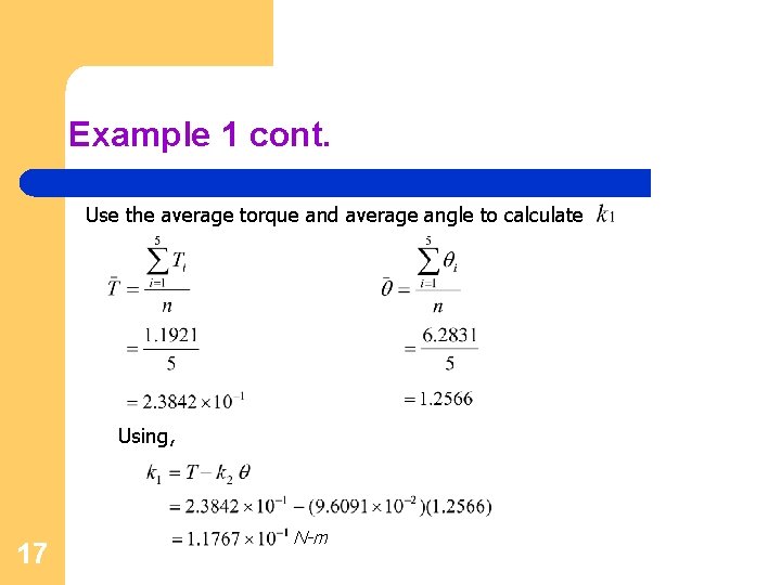
Example 1 cont. Use the average torque and average angle to calculate Using, 17 N-m

Example 1 Results Using linear regression, a trend line is found from the data 18 Figure. Linear regression of Torque versus Angle data Can you find the energy in the spring if it is twisted from 0 to 180 degrees?

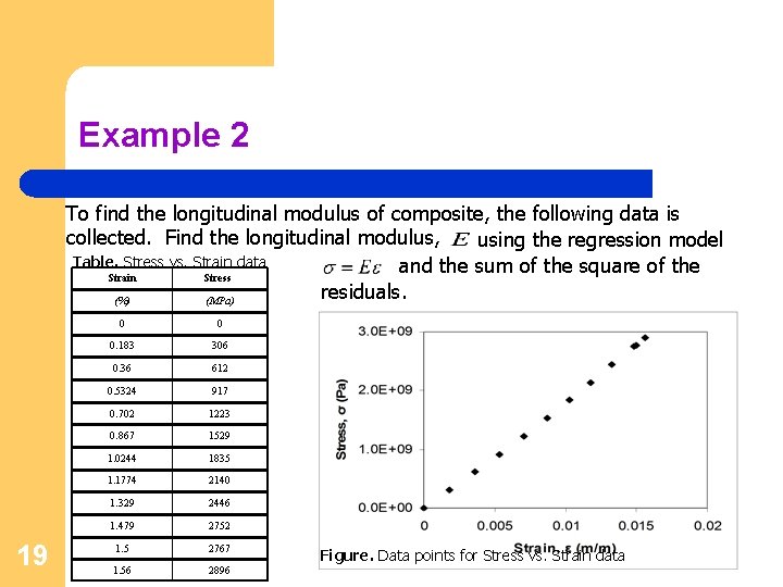
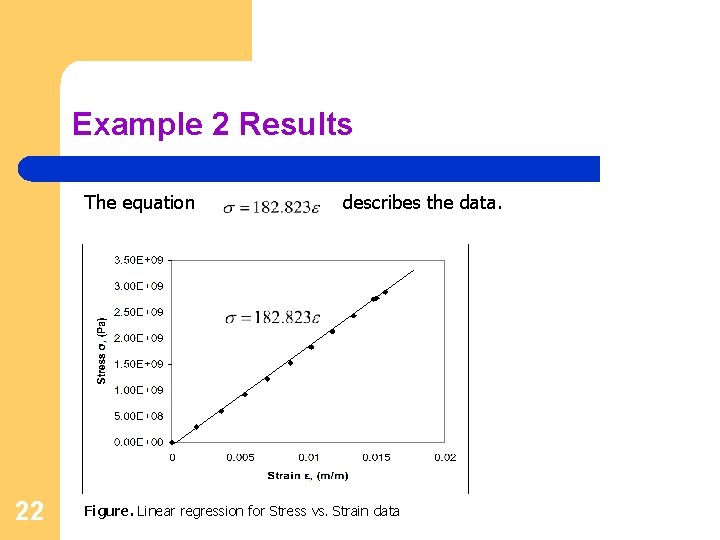
Example 2 To find the longitudinal modulus of composite, the following data is collected. Find the longitudinal modulus, using the regression model Table. Stress vs. Strain data and the sum of the square of the Strain Stress residuals. (%) (MPa) 19 0 0 0. 183 306 0. 36 612 0. 5324 917 0. 702 1223 0. 867 1529 1. 0244 1835 1. 1774 2140 1. 329 2446 1. 479 2752 1. 5 2767 1. 56 2896 Figure. Data points for Stress vs. Strain data

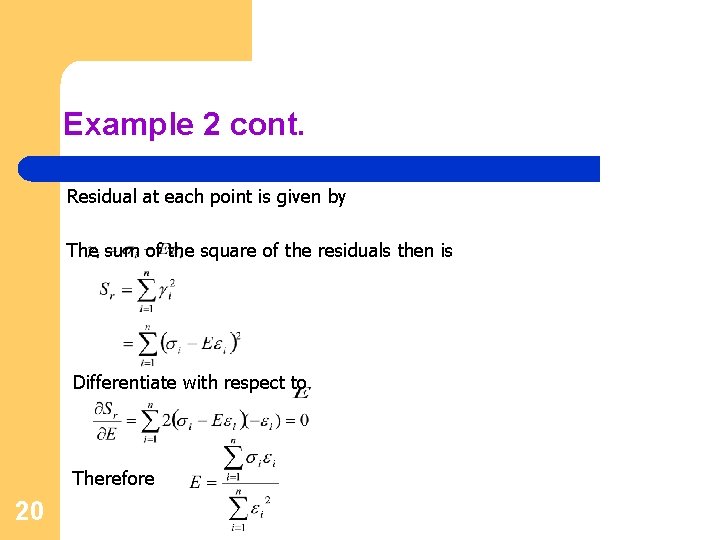
Example 2 cont. Residual at each point is given by The sum of the square of the residuals then is Differentiate with respect to Therefore 20

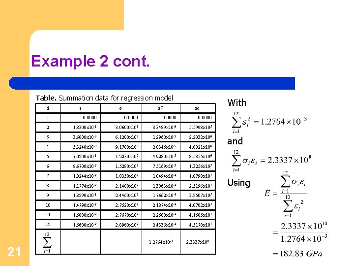
Example 2 cont. Table. Summation data for regression model i ε σ ε 2 1 0. 0000 2 1. 8300 x 10 -3 3. 0600 x 108 3. 3489 x 10 -6 5. 5998 x 105 3 3. 6000 x 10 -3 6. 1200 x 108 1. 2960 x 10 -5 2. 2032 x 106 4 5. 3240 x 10 -3 9. 1700 x 108 2. 8345 x 10 -5 4. 8821 x 106 5 7. 0200 x 10 -3 1. 2230 x 109 4. 9280 x 10 -5 8. 5855 x 106 6 8. 6700 x 10 -3 1. 5290 x 109 7. 5169 x 10 -5 1. 3256 x 107 7 1. 0244 x 10 -2 1. 8350 x 109 1. 0494 x 10 -4 1. 8798 x 107 8 1. 1774 x 10 -2 2. 1400 x 109 1. 3863 x 10 -4 2. 5196 x 107 9 1. 3290 x 10 -2 2. 4460 x 109 1. 7662 x 10 -4 3. 2507 x 107 10 1. 4790 x 10 -2 2. 7520 x 109 2. 1874 x 10 -4 4. 0702 x 107 11 1. 5000 x 10 -2 2. 7670 x 109 2. 2500 x 10 -4 4. 1505 x 107 12 1. 5600 x 10 -2 2. 8960 x 109 2. 4336 x 10 -4 4. 5178 x 107 1. 2764 x 10 -3 21 εσ 2. 3337 x 108 With and Using

Example 2 Results The equation 22 describes the data. Figure. Linear regression for Stress vs. Strain data

Nonlinear Regression Dr. A. Emamzadeh 23 6/6/2021

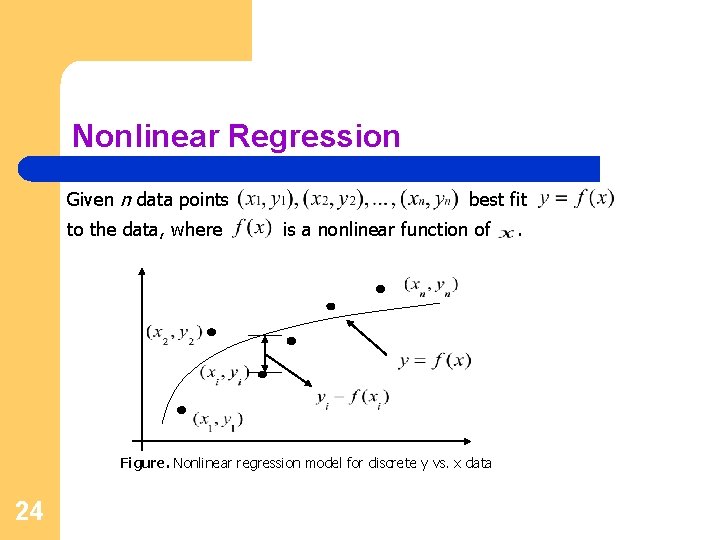
Nonlinear Regression Given n data points to the data, where best fit is a nonlinear function of Figure. Nonlinear regression model for discrete y vs. x data 24 .

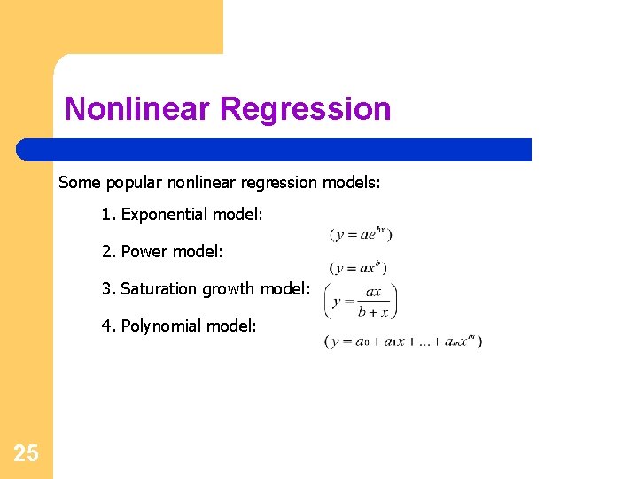
Nonlinear Regression Some popular nonlinear regression models: 1. Exponential model: 2. Power model: 3. Saturation growth model: 4. Polynomial model: 25

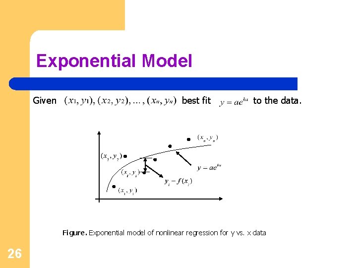
Exponential Model Given best fit to the data. Figure. Exponential model of nonlinear regression for y vs. x data 26

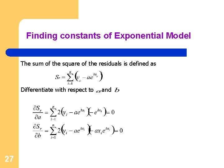
Finding constants of Exponential Model The sum of the square of the residuals is defined as Differentiate with respect to 27 and

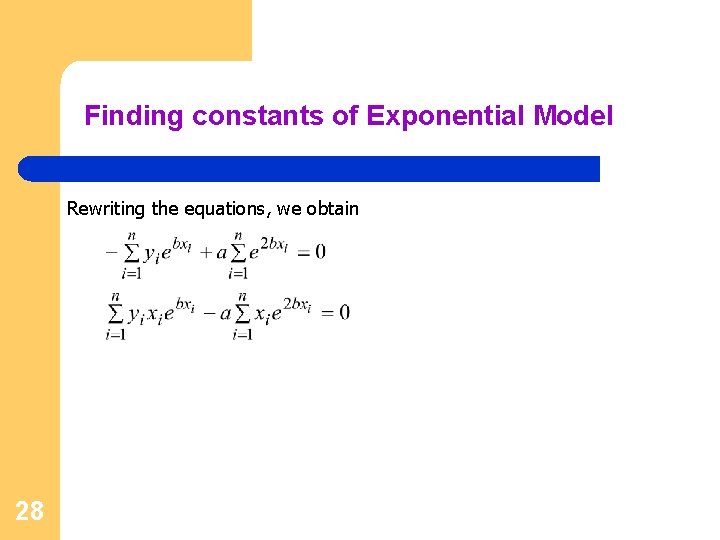
Finding constants of Exponential Model Rewriting the equations, we obtain 28

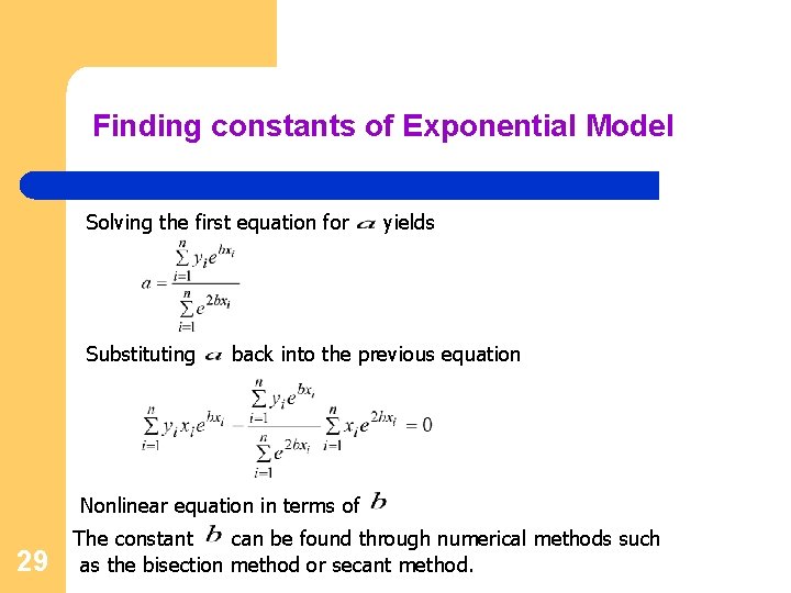
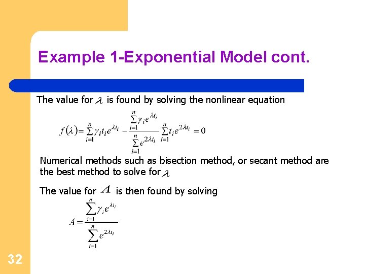
Finding constants of Exponential Model Solving the first equation for Substituting yields back into the previous equation Nonlinear equation in terms of 29 The constant can be found through numerical methods such as the bisection method or secant method.

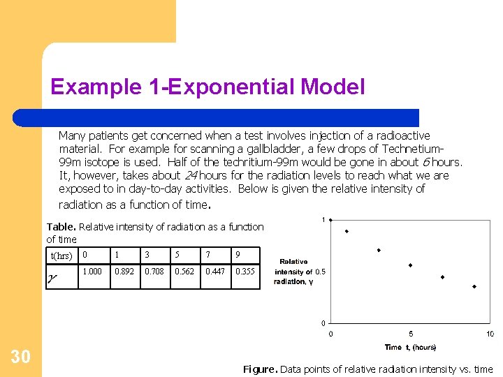
Example 1 -Exponential Model Many patients get concerned when a test involves injection of a radioactive material. For example for scanning a gallbladder, a few drops of Technetium 99 m isotope is used. Half of the techritium-99 m would be gone in about 6 hours. It, however, takes about 24 hours for the radiation levels to reach what we are exposed to in day-to-day activities. Below is given the relative intensity of radiation as a function of time. Table. Relative intensity of radiation as a function of time t(hrs) 30 0 1 3 5 7 9 1. 000 0. 892 0. 708 0. 562 0. 447 0. 355 Figure. Data points of relative radiation intensity vs. time

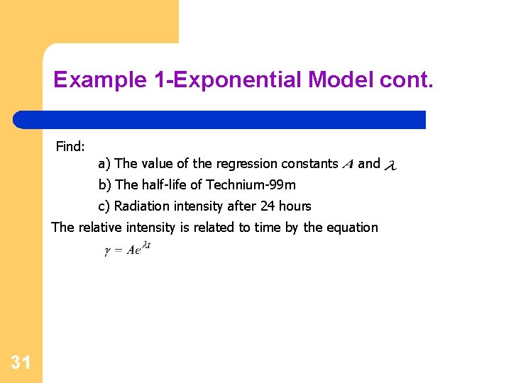
Example 1 -Exponential Model cont. Find: a) The value of the regression constants and b) The half-life of Technium-99 m c) Radiation intensity after 24 hours The relative intensity is related to time by the equation 31

Example 1 -Exponential Model cont. The value for is found by solving the nonlinear equation Numerical methods such as bisection method, or secant method are the best method to solve for The value for 32 is then found by solving

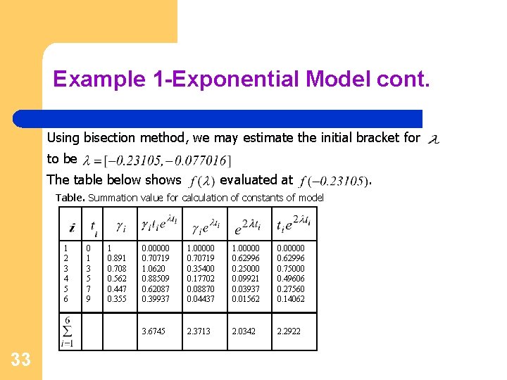
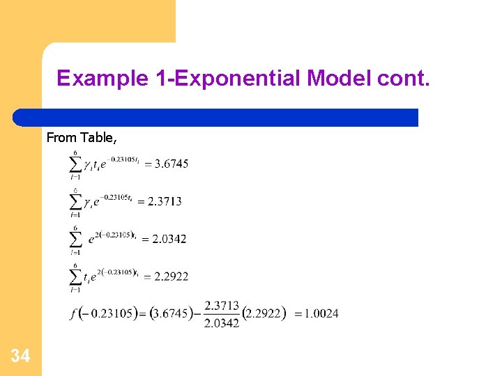
Example 1 -Exponential Model cont. Using bisection method, we may estimate the initial bracket for to be The table below shows evaluated at Table. Summation value for calculation of constants of model 1 2 3 4 5 6 33 0 1 3 5 7 9 1 0. 891 0. 708 0. 562 0. 447 0. 355 0. 00000 0. 70719 1. 0620 0. 88509 0. 62087 0. 39937 1. 00000 0. 70719 0. 35400 0. 17702 0. 08870 0. 04437 1. 00000 0. 62996 0. 25000 0. 09921 0. 03937 0. 01562 0. 00000 0. 62996 0. 75000 0. 49606 0. 27560 0. 14062 3. 6745 2. 3713 2. 0342 2. 2922 .

Example 1 -Exponential Model cont. From Table, 34

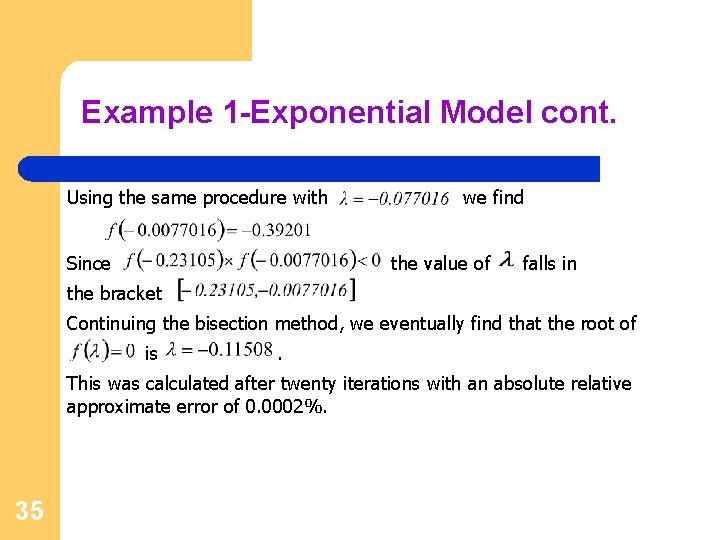
Example 1 -Exponential Model cont. Using the same procedure with Since we find the value of falls in the bracket Continuing the bisection method, we eventually find that the root of is . This was calculated after twenty iterations with an absolute relative approximate error of 0. 0002%. 35

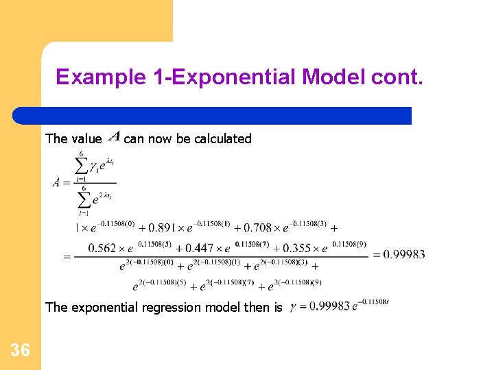
Example 1 -Exponential Model cont. The value can now be calculated The exponential regression model then is 36

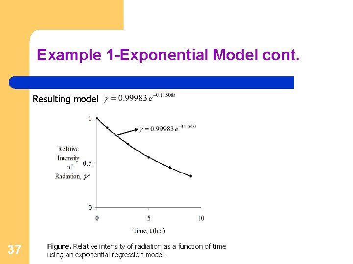
Example 1 -Exponential Model cont. Resulting model 37 Figure. Relative intensity of radiation as a function of time using an exponential regression model.

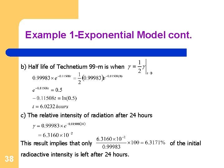
Example 1 -Exponential Model cont. b) Half life of Technetium 99 -m is when c) The relative intensity of radiation after 24 hours This result implies that only 38 radioactive intensity is left after 24 hours. of the initial

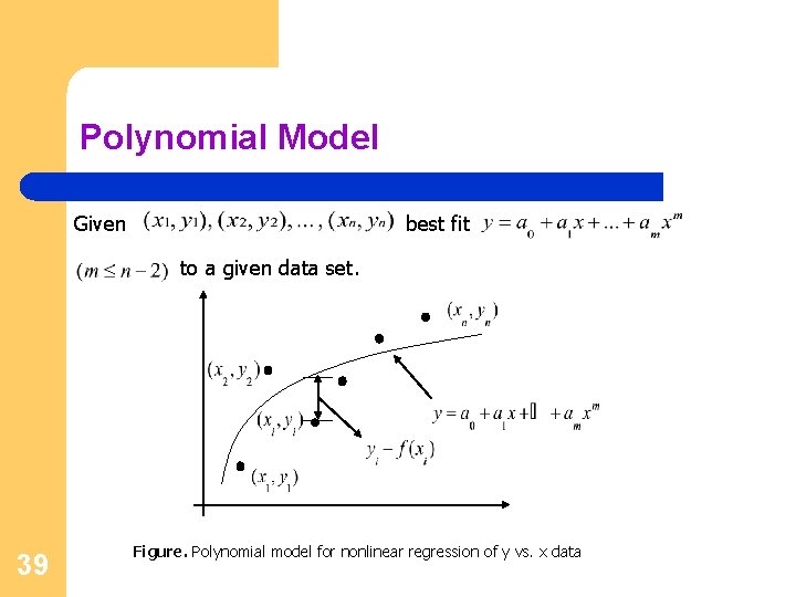
Polynomial Model Given best fit to a given data set. 39 Figure. Polynomial model for nonlinear regression of y vs. x data

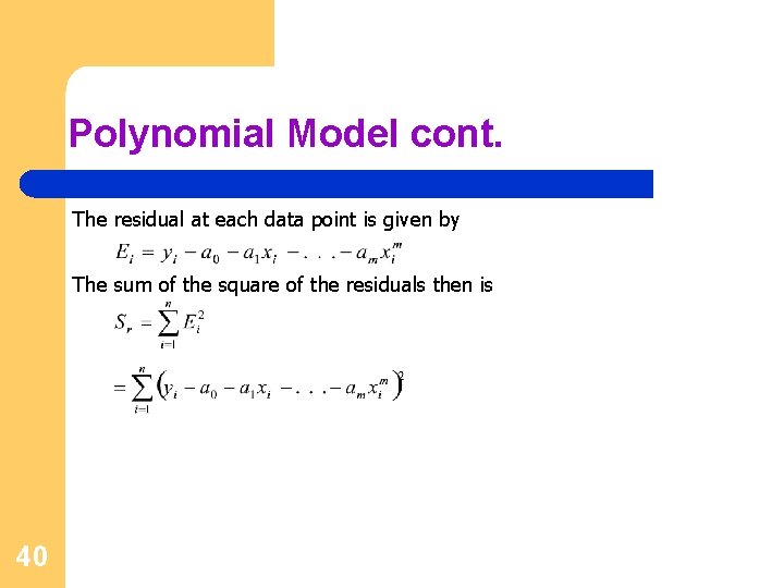
Polynomial Model cont. The residual at each data point is given by The sum of the square of the residuals then is 40

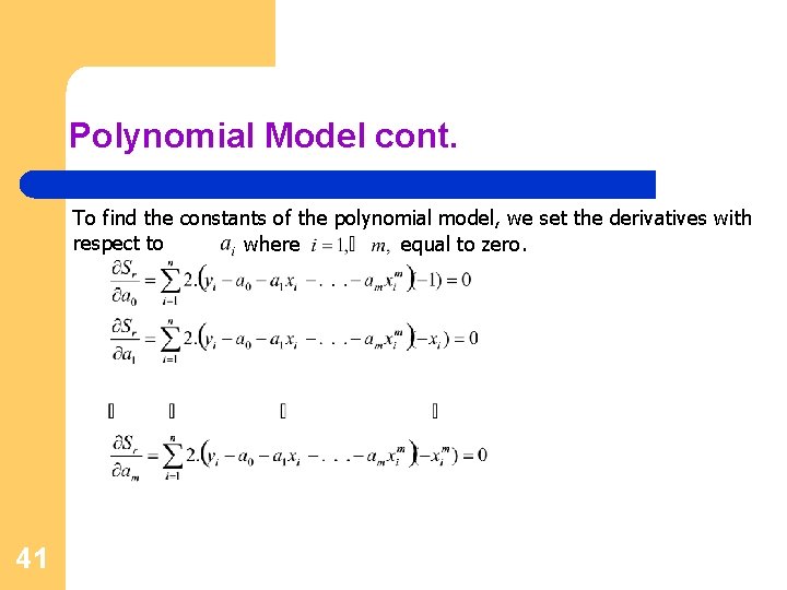
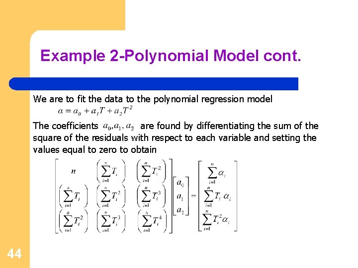
Polynomial Model cont. To find the constants of the polynomial model, we set the derivatives with respect to where equal to zero. 41

Polynomial Model cont. These equations in matrix form are given by The above equations are then solved for 42

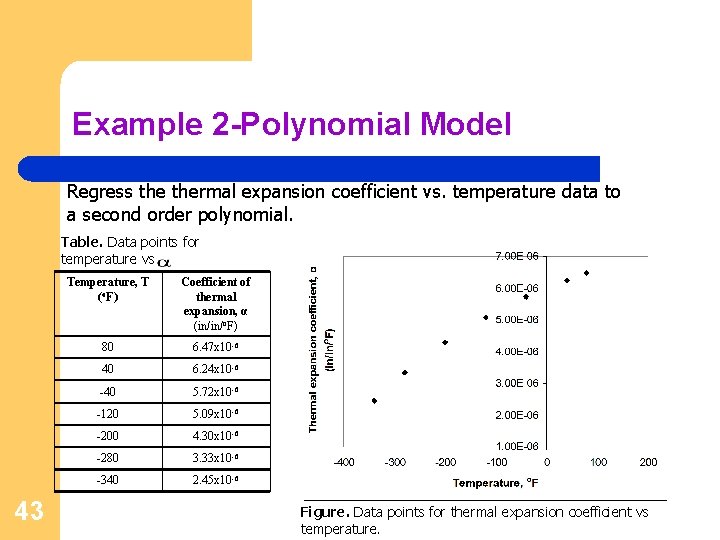
Example 2 -Polynomial Model Regress thermal expansion coefficient vs. temperature data to a second order polynomial. Table. Data points for temperature vs 43 Temperature, T (o. F) Coefficient of thermal expansion, α (in/in/o. F) 80 6. 47 x 10 -6 40 6. 24 x 10 -6 -40 5. 72 x 10 -6 -120 5. 09 x 10 -6 -200 4. 30 x 10 -6 -280 3. 33 x 10 -6 -340 2. 45 x 10 -6 Figure. Data points for thermal expansion coefficient vs temperature.

Example 2 -Polynomial Model cont. We are to fit the data to the polynomial regression model The coefficients are found by differentiating the sum of the square of the residuals with respect to each variable and setting the values equal to zero to obtain 44

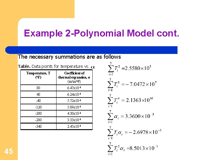
Example 2 -Polynomial Model cont. The necessary summations are as follows Table. Data points for temperature vs. 45 Temperature, T (o. F) Coefficient of thermal expansion, α (in/in/o. F) 80 6. 47 x 10 -6 40 6. 24 x 10 -6 -40 5. 72 x 10 -6 -120 5. 09 x 10 -6 -200 4. 30 x 10 -6 -280 3. 33 x 10 -6 -340 2. 45 x 10 -6

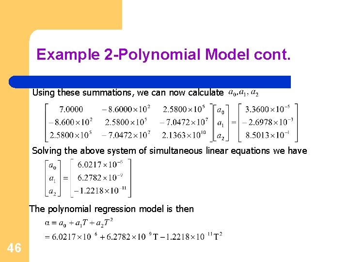
Example 2 -Polynomial Model cont. Using these summations, we can now calculate Solving the above system of simultaneous linear equations we have The polynomial regression model is then 46

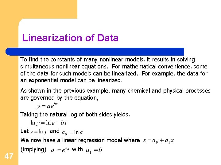
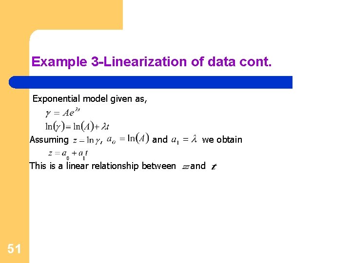
Linearization of Data To find the constants of many nonlinear models, it results in solving simultaneous nonlinear equations. For mathematical convenience, some of the data for such models can be linearized. For example, the data for an exponential model can be linearized. As shown in the previous example, many chemical and physical processes are governed by the equation, Taking the natural log of both sides yields, Let and We now have a linear regression model where 47 (implying) with

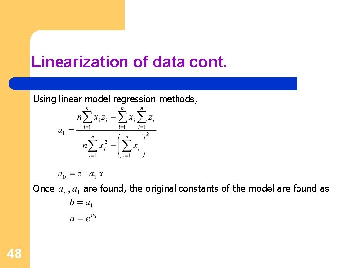
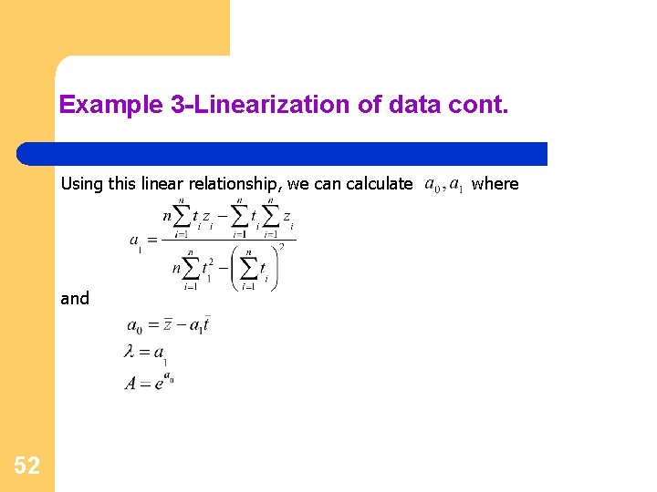
Linearization of data cont. Using linear model regression methods, Once 48 are found, the original constants of the model are found as

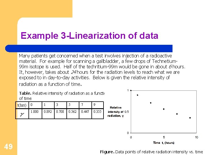
Example 3 -Linearization of data Many patients get concerned when a test involves injection of a radioactive material. For example for scanning a gallbladder, a few drops of Technetium 99 m isotope is used. Half of the techritium-99 m would be gone in about 6 hours. It, however, takes about 24 hours for the radiation levels to reach what we are exposed to in day-to-day activities. Below is given the relative intensity of radiation as a function of time. Table. Relative intensity of radiation as a function of time t(hrs) 49 0 1 3 5 7 9 1. 000 0. 892 0. 708 0. 562 0. 447 0. 355 Figure. Data points of relative radiation intensity vs. time

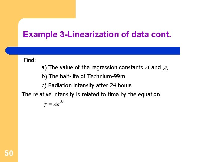
Example 3 -Linearization of data cont. Find: a) The value of the regression constants and b) The half-life of Technium-99 m c) Radiation intensity after 24 hours The relative intensity is related to time by the equation 50

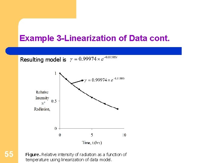
Example 3 -Linearization of data cont. Exponential model given as, Assuming , and This is a linear relationship between 51 we obtain and

Example 3 -Linearization of data cont. Using this linear relationship, we can calculate and 52 where

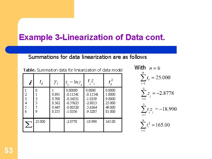
Example 3 -Linearization of Data cont. Summations for data linearization are as follows Table. Summation data for linearization of data model 1 2 3 4 5 6 0 1 3 5 7 9 25. 000 53 1 0. 891 0. 708 0. 562 0. 447 0. 355 0. 00000 -0. 11541 -0. 34531 -0. 57625 -0. 80520 -1. 0356 0. 0000 -0. 11541 -1. 0359 -2. 8813 -5. 6364 -9. 3207 0. 0000 1. 0000 9. 0000 25. 000 49. 000 81. 000 -2. 8778 -18. 990 165. 00 With

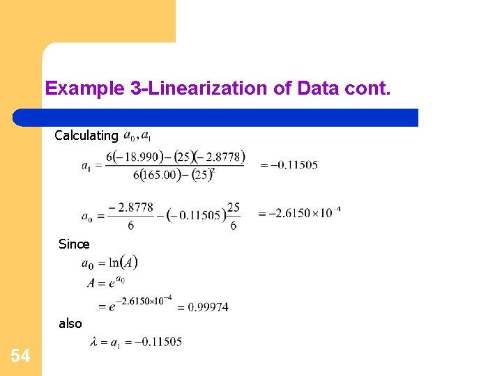
Example 3 -Linearization of Data cont. Calculating Since also 54

Example 3 -Linearization of Data cont. Resulting model is 55 Figure. Relative intensity of radiation as a function of temperature using linearization of data model.

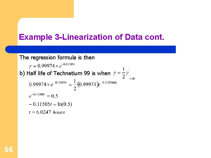
Example 3 -Linearization of Data cont. The regression formula is then b) Half life of Technetium 99 is when 56

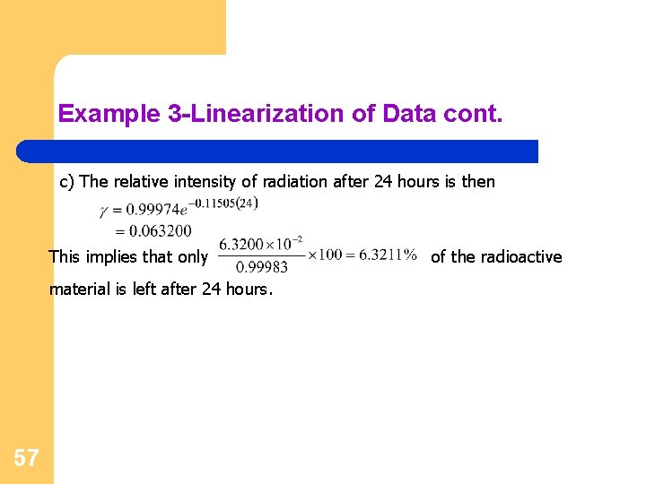
Example 3 -Linearization of Data cont. c) The relative intensity of radiation after 24 hours is then This implies that only material is left after 24 hours. 57 of the radioactive

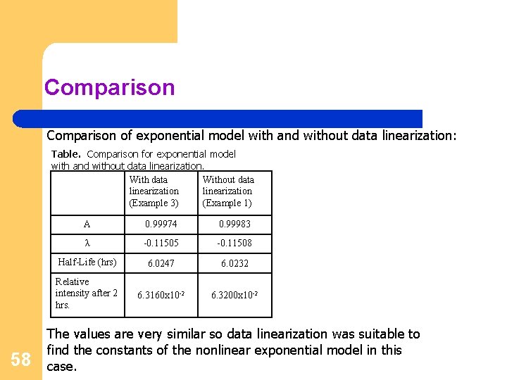
Comparison of exponential model with and without data linearization: Table. Comparison for exponential model with and without data linearization. With data Without data linearization (Example 3) (Example 1) 58 A 0. 99974 0. 99983 λ -0. 11505 -0. 11508 Half-Life (hrs) 6. 0247 6. 0232 Relative intensity after 2 hrs. 6. 3160 x 10 -2 6. 3200 x 10 -2 The values are very similar so data linearization was suitable to find the constants of the nonlinear exponential model in this case.