Linear Regression Computer Engineering Majors Authors Autar Kaw

Linear Regression Computer Engineering Majors Authors: Autar Kaw, Luke Snyder http: //numericalmethods. eng. usf. edu Transforming Numerical Methods Education for STEM Undergraduates 10/23/2021 http: //numericalmethods. eng. usf. edu 1

Linear Regression http: //numericalmethods. eng. usf. edu

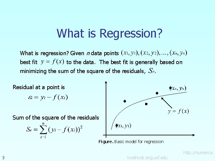
What is Regression? What is regression? Given n data points best fit to the data. The best fit is generally based on minimizing the sum of the square of the residuals, . Residual at a point is Sum of the square of the residuals Figure. Basic model for regression 3 lmethods. eng. usf. edu http: //numerica

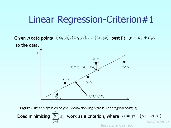
Linear Regression-Criterion#1 Given n data points best fit to the data. y x Figure. Linear regression of y vs. x data showing residuals at a typical point, xi. Does minimizing 4 work as a criterion, where lmethods. eng. usf. edu http: //numerica

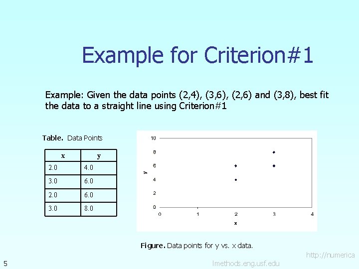
Example for Criterion#1 Example: Given the data points (2, 4), (3, 6), (2, 6) and (3, 8), best fit the data to a straight line using Criterion#1 Table. Data Points x y 2. 0 4. 0 3. 0 6. 0 2. 0 6. 0 3. 0 8. 0 Figure. Data points for y vs. x data. 5 lmethods. eng. usf. edu http: //numerica

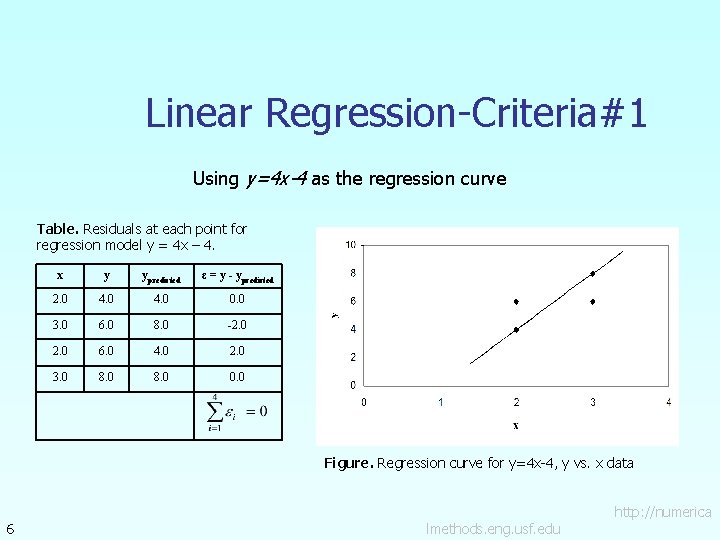
Linear Regression-Criteria#1 Using y=4 x-4 as the regression curve Table. Residuals at each point for regression model y = 4 x – 4. x y ypredicted ε = y - ypredicted 2. 0 4. 0 0. 0 3. 0 6. 0 8. 0 -2. 0 6. 0 4. 0 2. 0 3. 0 8. 0 0. 0 Figure. Regression curve for y=4 x-4, y vs. x data 6 lmethods. eng. usf. edu http: //numerica

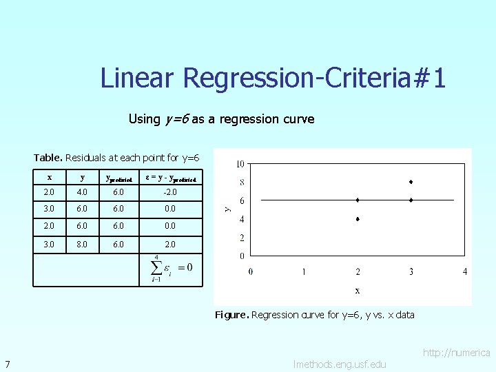
Linear Regression-Criteria#1 Using y=6 as a regression curve Table. Residuals at each point for y=6 x y ypredicted ε = y - ypredicted 2. 0 4. 0 6. 0 -2. 0 3. 0 6. 0 0. 0 2. 0 6. 0 0. 0 3. 0 8. 0 6. 0 2. 0 Figure. Regression curve for y=6, y vs. x data 7 lmethods. eng. usf. edu http: //numerica

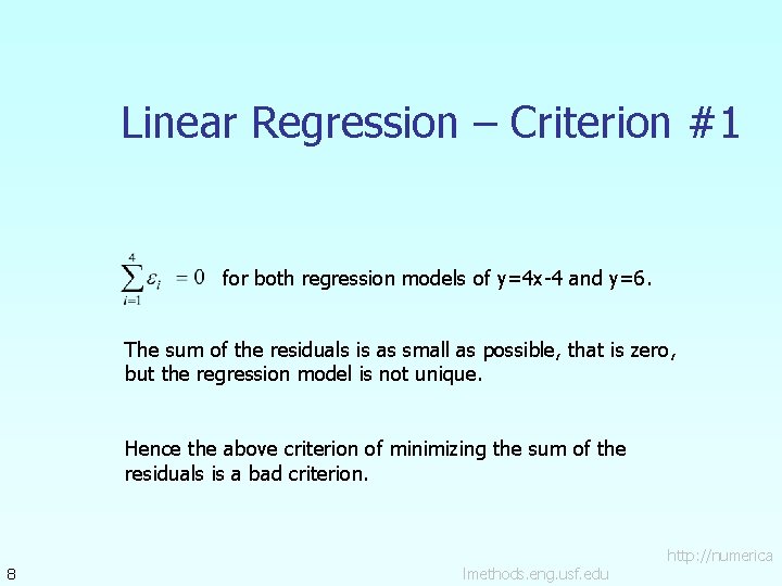
Linear Regression – Criterion #1 for both regression models of y=4 x-4 and y=6. The sum of the residuals is as small as possible, that is zero, but the regression model is not unique. Hence the above criterion of minimizing the sum of the residuals is a bad criterion. 8 lmethods. eng. usf. edu http: //numerica

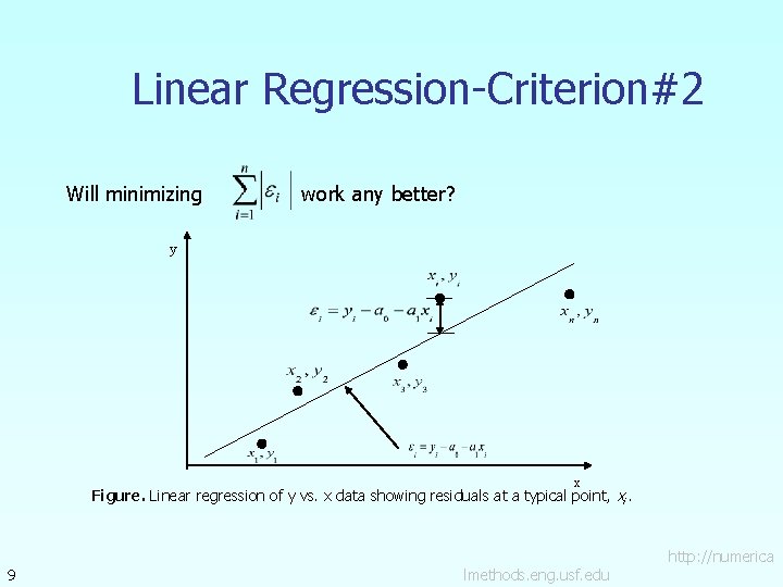
Linear Regression-Criterion#2 Will minimizing work any better? y x Figure. Linear regression of y vs. x data showing residuals at a typical point, xi. 9 lmethods. eng. usf. edu http: //numerica

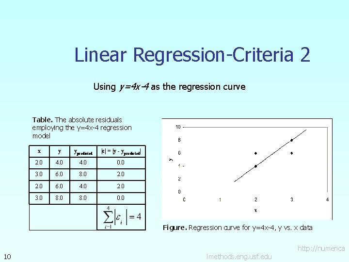
Linear Regression-Criteria 2 Using y=4 x-4 as the regression curve Table. The absolute residuals employing the y=4 x-4 regression model x y ypredicted |ε| = |y - ypredicted| 2. 0 4. 0 0. 0 3. 0 6. 0 8. 0 2. 0 6. 0 4. 0 2. 0 3. 0 8. 0 0. 0 Figure. Regression curve for y=4 x-4, y vs. x data 10 lmethods. eng. usf. edu http: //numerica

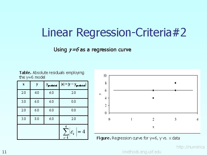
Linear Regression-Criteria#2 Using y=6 as a regression curve Table. Absolute residuals employing the y=6 model x y ypredicted |ε| = |y – ypredicted| 2. 0 4. 0 6. 0 2. 0 3. 0 6. 0 0. 0 2. 0 6. 0 0. 0 3. 0 8. 0 6. 0 2. 0 Figure. Regression curve for y=6, y vs. x data 11 lmethods. eng. usf. edu http: //numerica

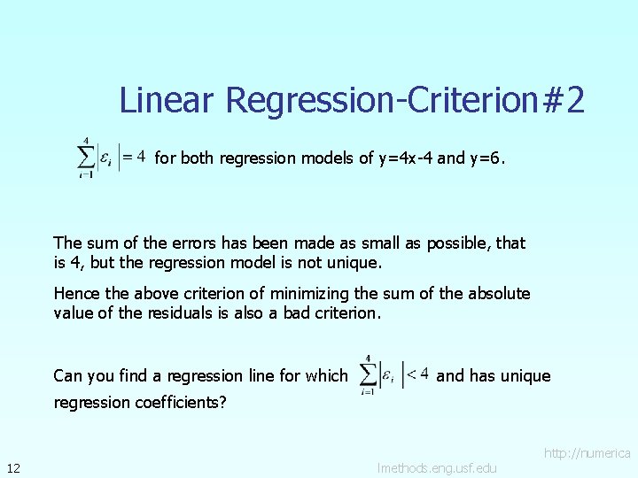
Linear Regression-Criterion#2 for both regression models of y=4 x-4 and y=6. The sum of the errors has been made as small as possible, that is 4, but the regression model is not unique. Hence the above criterion of minimizing the sum of the absolute value of the residuals is also a bad criterion. Can you find a regression line for which and has unique regression coefficients? 12 lmethods. eng. usf. edu http: //numerica

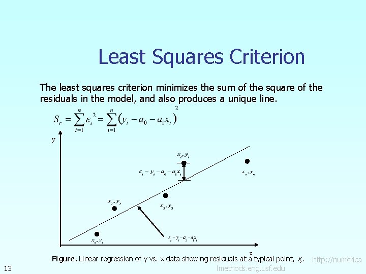
Least Squares Criterion The least squares criterion minimizes the sum of the square of the residuals in the model, and also produces a unique line. y x 13 Figure. Linear regression of y vs. x data showing residuals at a typical point, xi. lmethods. eng. usf. edu http: //numerica

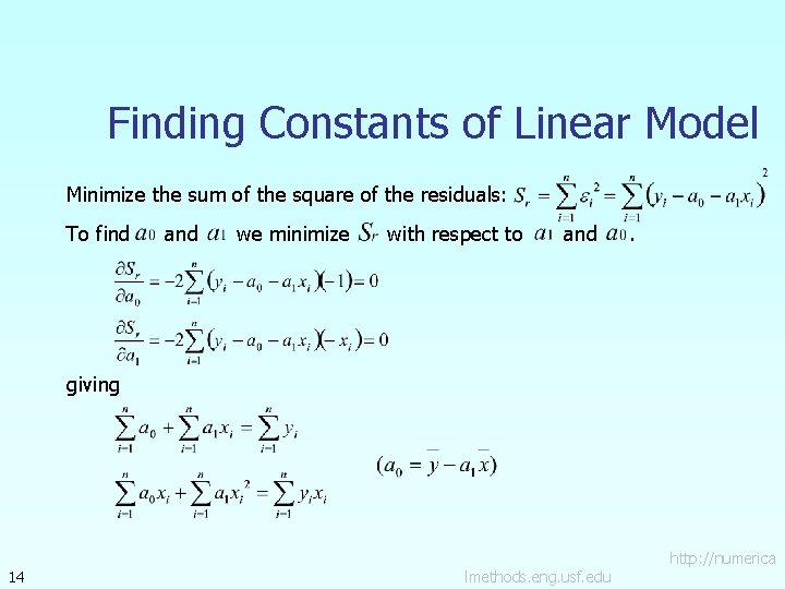
Finding Constants of Linear Model Minimize the sum of the square of the residuals: To find and we minimize with respect to and . giving 14 lmethods. eng. usf. edu http: //numerica

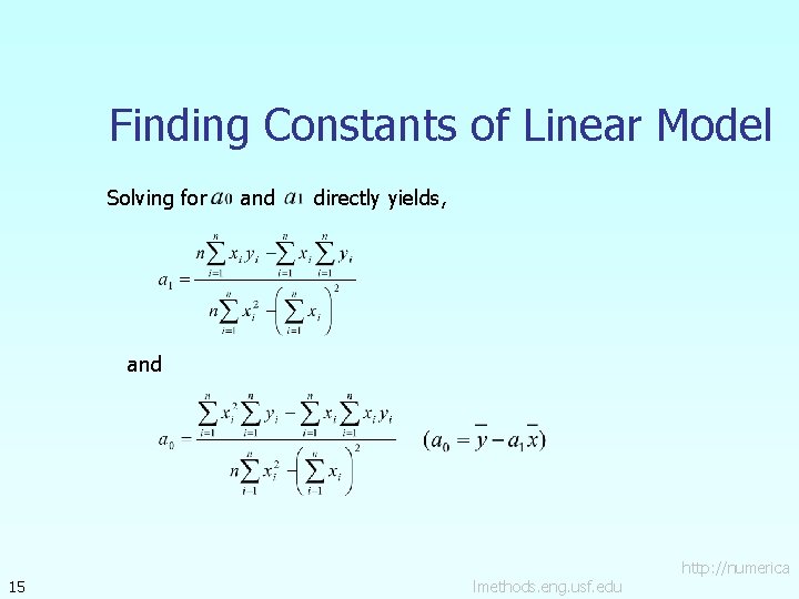
Finding Constants of Linear Model Solving for and directly yields, and 15 lmethods. eng. usf. edu http: //numerica

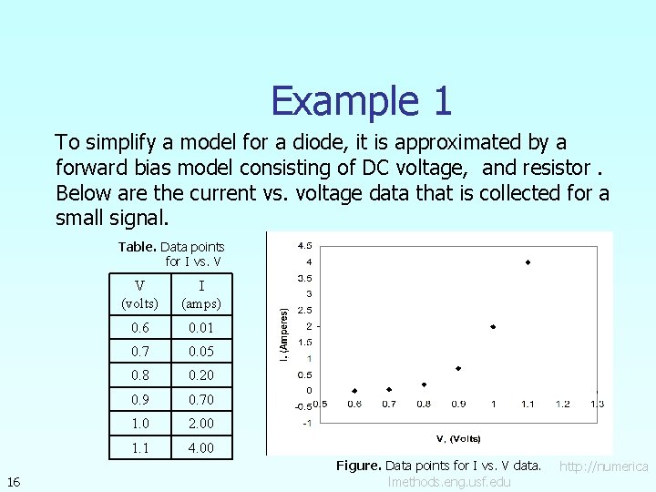
Example 1 To simplify a model for a diode, it is approximated by a forward bias model consisting of DC voltage, and resistor. Below are the current vs. voltage data that is collected for a small signal. Table. Data points for I vs. V 16 V (volts) I (amps) 0. 6 0. 01 0. 7 0. 05 0. 8 0. 20 0. 9 0. 70 1. 0 2. 00 1. 1 4. 00 Figure. Data points for I vs. V data. lmethods. eng. usf. edu http: //numerica

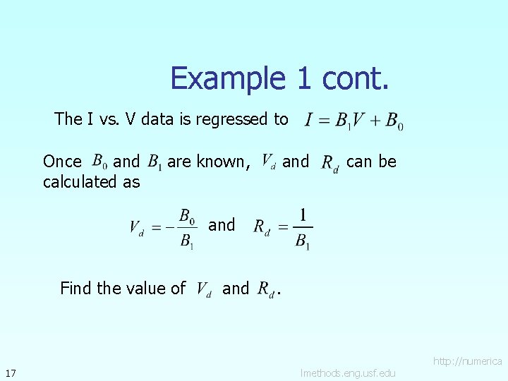
Example 1 cont. The I vs. V data is regressed to Once and calculated as are known, and can be and Find the value of 17 and . lmethods. eng. usf. edu http: //numerica

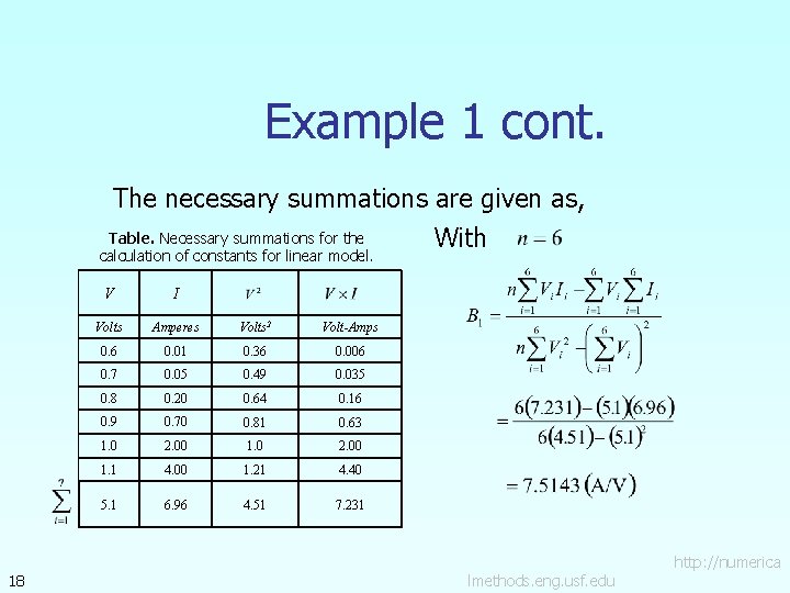
Example 1 cont. The necessary summations are given as, Table. Necessary summations for the With calculation of constants for linear model. 18 V I Volts Amperes Volts 2 Volt-Amps 0. 6 0. 01 0. 36 0. 006 0. 7 0. 05 0. 49 0. 035 0. 8 0. 20 0. 64 0. 16 0. 9 0. 70 0. 81 0. 63 1. 0 2. 00 1. 1 4. 00 1. 21 4. 40 5. 1 6. 96 4. 51 7. 231 lmethods. eng. usf. edu http: //numerica

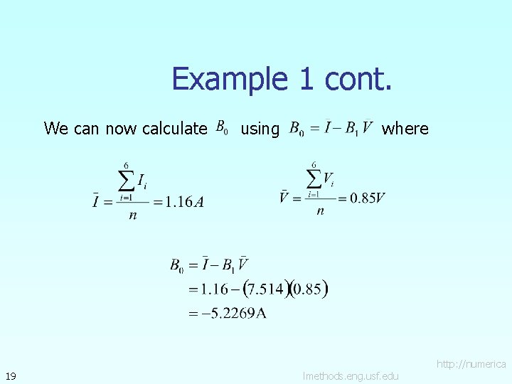
Example 1 cont. We can now calculate 19 using where lmethods. eng. usf. edu http: //numerica

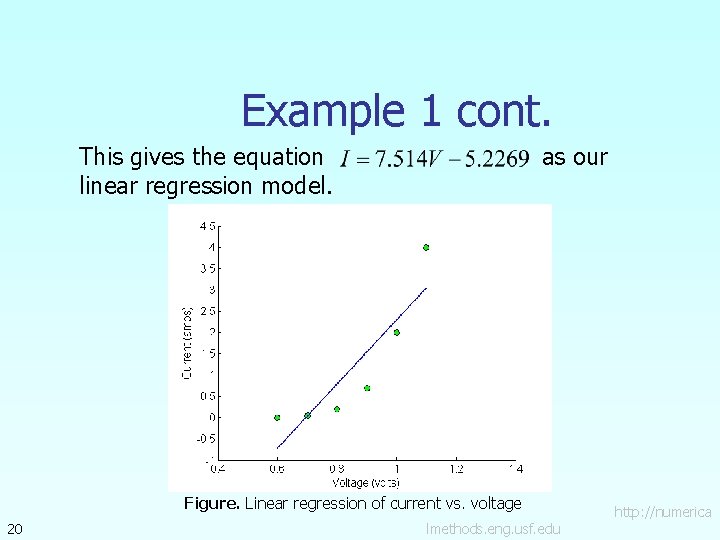
Example 1 cont. This gives the equation linear regression model. as our Figure. Linear regression of current vs. voltage 20 lmethods. eng. usf. edu http: //numerica

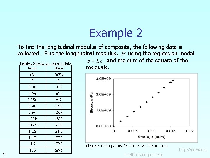
Example 2 To find the longitudinal modulus of composite, the following data is using the regression model collected. Find the longitudinal modulus, and the sum of the square of the Table. Stress vs. Strain data Strain Stress residuals. 21 (%) (MPa) 0 0 0. 183 306 0. 36 612 0. 5324 917 0. 702 1223 0. 867 1529 1. 0244 1835 1. 1774 2140 1. 329 2446 1. 479 2752 1. 5 2767 1. 56 2896 Figure. Data points for Stress vs. Strain data lmethods. eng. usf. edu http: //numerica

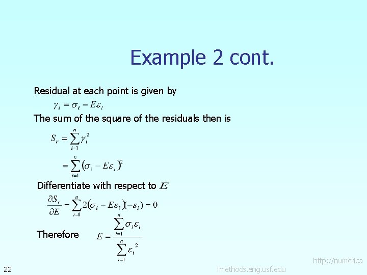
Example 2 cont. Residual at each point is given by The sum of the square of the residuals then is Differentiate with respect to Therefore 22 lmethods. eng. usf. edu http: //numerica

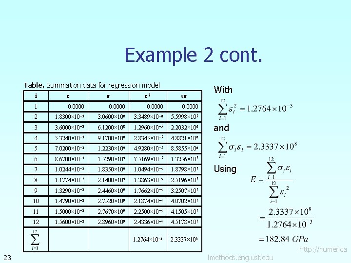
Example 2 cont. Table. Summation data for regression model 23 i ε σ ε 2 εσ 1 0. 0000 2 1. 8300× 10− 3 3. 0600× 108 3. 3489× 10− 6 5. 5998× 105 3 3. 6000× 10− 3 6. 1200× 108 1. 2960× 10− 5 2. 2032× 106 4 5. 3240× 10− 3 9. 1700× 108 2. 8345× 10− 5 4. 8821× 106 5 7. 0200× 10− 3 1. 2230× 109 4. 9280× 10− 5 8. 5855× 106 6 8. 6700× 10− 3 1. 5290× 109 7. 5169× 10− 5 1. 3256× 107 7 1. 0244× 10− 2 1. 8350× 109 1. 0494× 10− 4 1. 8798× 107 8 1. 1774× 10− 2 2. 1400× 109 1. 3863× 10− 4 2. 5196× 107 9 1. 3290× 10− 2 2. 4460× 109 1. 7662× 10− 4 3. 2507× 107 10 1. 4790× 10− 2 2. 7520× 109 2. 1874× 10− 4 4. 0702× 107 11 1. 5000× 10− 2 2. 7670× 109 2. 2500× 10− 4 4. 1505× 107 12 1. 5600× 10− 2 2. 8960× 109 2. 4336× 10− 4 4. 5178× 107 1. 2764× 10− 3 2. 3337× 108 With and Using lmethods. eng. usf. edu http: //numerica

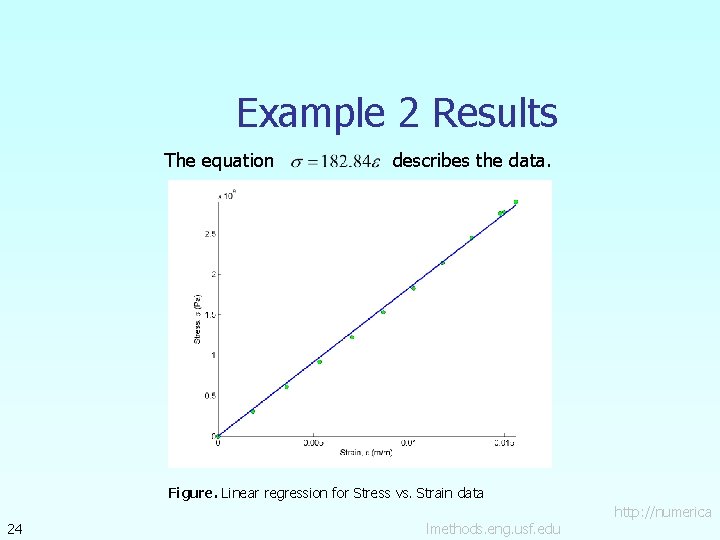
Example 2 Results The equation describes the data. Figure. Linear regression for Stress vs. Strain data 24 lmethods. eng. usf. edu http: //numerica

Additional Resources For all resources on this topic such as digital audiovisual lectures, primers, textbook chapters, multiple-choice tests, worksheets in MATLAB, MATHEMATICA, Math. Cad and MAPLE, blogs, related physical problems, please visit http: //numericalmethods. eng. usf. edu/topics/linear_regr ession. html

THE END http: //numericalmethods. eng. usf. edu