LINEAR PROGRAMMING OUTLINE v Key characteristics and applications

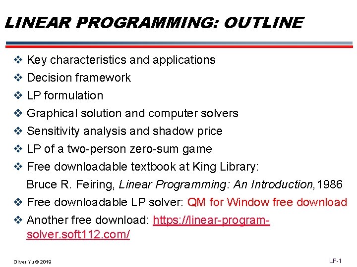
LINEAR PROGRAMMING: OUTLINE v Key characteristics and applications v Decision framework v LP formulation v Graphical solution and computer solvers v Sensitivity analysis and shadow price v LP of a two-person zero-sum game v Free downloadable textbook at King Library: Bruce R. Feiring, Linear Programming: An Introduction, 1986 v Free downloadable LP solver: QM for Window free download v Another free download: https: //linear-programsolver. soft 112. com/ Oliver Yu © 2019 LP-1

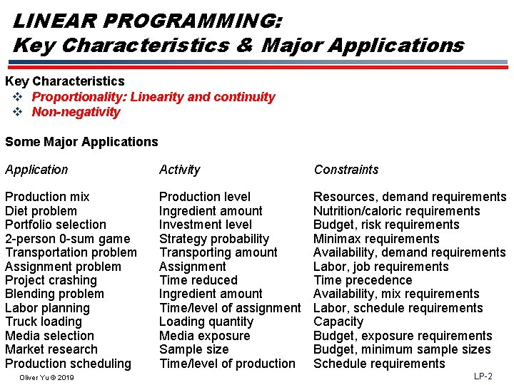
LINEAR PROGRAMMING: Key Characteristics & Major Applications Key Characteristics v Proportionality: Linearity and continuity v Non-negativity Some Major Applications Application Activity Constraints Production mix Diet problem Portfolio selection 2 -person 0 -sum game Transportation problem Assignment problem Project crashing Blending problem Labor planning Truck loading Media selection Market research Production scheduling Production level Ingredient amount Investment level Strategy probability Transporting amount Assignment Time reduced Ingredient amount Time/level of assignment Loading quantity Media exposure Sample size Time/level of production Resources, demand requirements Nutrition/caloric requirements Budget, risk requirements Minimax requirements Availability, demand requirements Labor, job requirements Time precedence Availability, mix requirements Labor, schedule requirements Capacity Budget, exposure requirements Budget, minimum sample sizes Schedule requirements Oliver Yu © 2019 LP-2

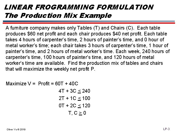
LINEAR FROGRAMMING FORMULATION The Production Mix Example A furniture company makes only Tables (T) and Chairs (C). Each table produces $60 net profit and each chair produces $40 net profit. Each table takes 4 hours of carpenter’s time, 2 hours of painter’s time, and 0 hour of metal worker’s time; each chair takes 3 hours of carpenter’s time, 1 hour of painter’s time, and 2 hours of metal worker’s time. Each week, 240 hours of carpenter’s time, 100 hours of painter’s time, and 120 hours of metal worker’s time are available. Find the production mix of tables and chairs that will maximize the weekly net profit P. Maximize V = Profit = 60 T + 40 C 4 T + 3 C < 240 2 T + 1 C < 100 0 T + 2 C < 120 T, C > 0 Oliver Yu © 2019 LP-3

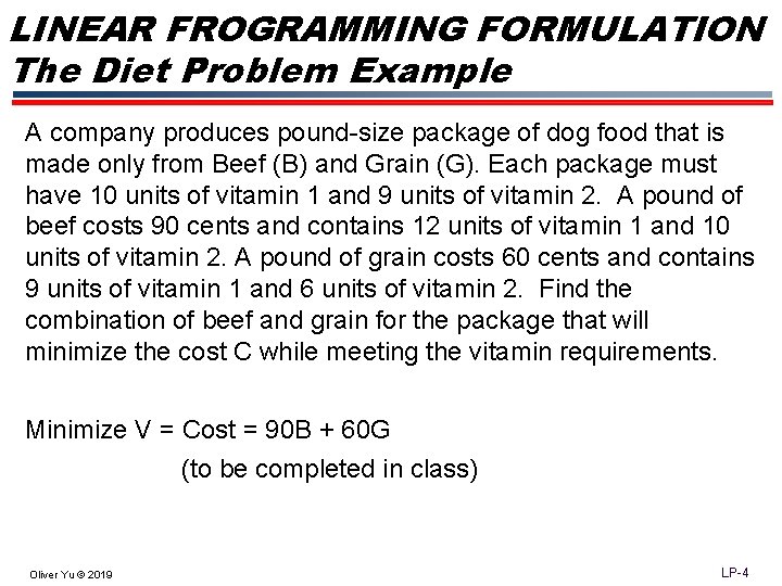
LINEAR FROGRAMMING FORMULATION The Diet Problem Example A company produces pound-size package of dog food that is made only from Beef (B) and Grain (G). Each package must have 10 units of vitamin 1 and 9 units of vitamin 2. A pound of beef costs 90 cents and contains 12 units of vitamin 1 and 10 units of vitamin 2. A pound of grain costs 60 cents and contains 9 units of vitamin 1 and 6 units of vitamin 2. Find the combination of beef and grain for the package that will minimize the cost C while meeting the vitamin requirements. Minimize V = Cost = 90 B + 60 G (to be completed in class) Oliver Yu © 2019 LP-4

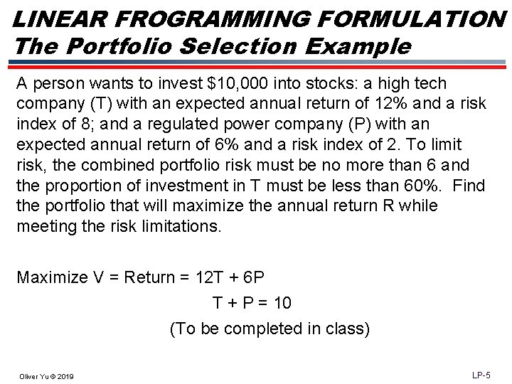
LINEAR FROGRAMMING FORMULATION The Portfolio Selection Example A person wants to invest $10, 000 into stocks: a high tech company (T) with an expected annual return of 12% and a risk index of 8; and a regulated power company (P) with an expected annual return of 6% and a risk index of 2. To limit risk, the combined portfolio risk must be no more than 6 and the proportion of investment in T must be less than 60%. Find the portfolio that will maximize the annual return R while meeting the risk limitations. Maximize V = Return = 12 T + 6 P T + P = 10 (To be completed in class) Oliver Yu © 2019 LP-5

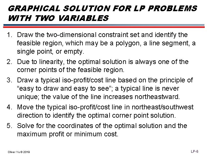
GRAPHICAL SOLUTION FOR LP PROBLEMS WITH TWO VARIABLES 1. Draw the two-dimensional constraint set and identify the feasible region, which may be a polygon, a line segment, a single point, or empty. 2. Due to linearity, the optimal solution is always one of the corner points of the feasible region. 3. Draw a typical iso-profit/cost line based on the principle of “easy to draw and easy to see”; a typical line is never unique; the value of the line increases northeastward. 4. Move the typical iso-profit/cost line in northeast/southwest direction to identify the optimal corner point solution. 5. Solve for the coordinates of the optimal solution and the maximum profit or minimum cost. Oliver Yu © 2019 LP-6

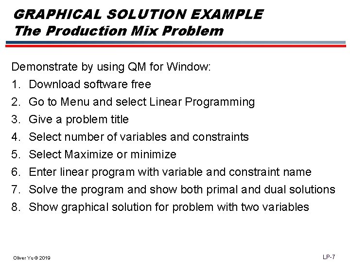
GRAPHICAL SOLUTION EXAMPLE The Production Mix Problem Demonstrate by using QM for Window: 1. Download software free 2. 3. 4. 5. 6. 7. 8. Go to Menu and select Linear Programming Give a problem title Select number of variables and constraints Select Maximize or minimize Enter linear program with variable and constraint name Solve the program and show both primal and dual solutions Show graphical solution for problem with two variables Oliver Yu © 2019 LP-7

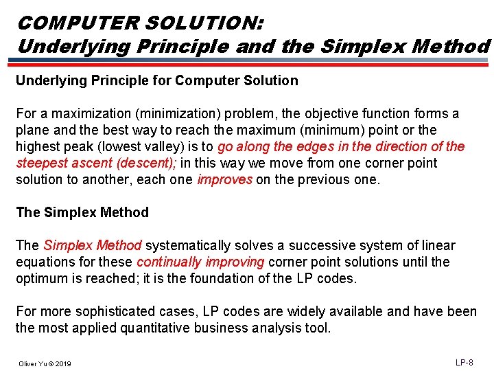
COMPUTER SOLUTION: Underlying Principle and the Simplex Method Underlying Principle for Computer Solution For a maximization (minimization) problem, the objective function forms a plane and the best way to reach the maximum (minimum) point or the highest peak (lowest valley) is to go along the edges in the direction of the steepest ascent (descent); in this way we move from one corner point solution to another, each one improves on the previous one. The Simplex Method systematically solves a successive system of linear equations for these continually improving corner point solutions until the optimum is reached; it is the foundation of the LP codes. For more sophisticated cases, LP codes are widely available and have been the most applied quantitative business analysis tool. Oliver Yu © 2019 LP-8

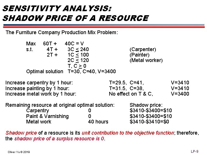
SENSITIVITY ANALYSIS: SHADOW PRICE OF A RESOURCE The Furniture Company Production Mix Problem: Max s. t. 60 T + 4 T + 2 T + 40 C = V 3 C < 240 1 C < 100 2 C < 120 T, C > 0 Optimal solution T=30, C=40, V=3400 Increase carpentry by 1 hour: Increase painting by 1 hour: Increase metal work by 1 hour: (Carpenter) (Painter) (Metal worker) T=29. 5, C=41, T=31. 5, C=38, No effect on T & C, Remaining resource at original optimal solution: Carpentry 0 Paint & Varnishing 0 Metal work 40 hours V=3410 V=3400 Shadow price: $3410 -$3400=$10 $3410 -$3410=$0 Shadow price of a resource is its unit contribution to the objective function; therefore, the shadow price of a surplus resource is 0. Oliver Yu © 2019 LP-9

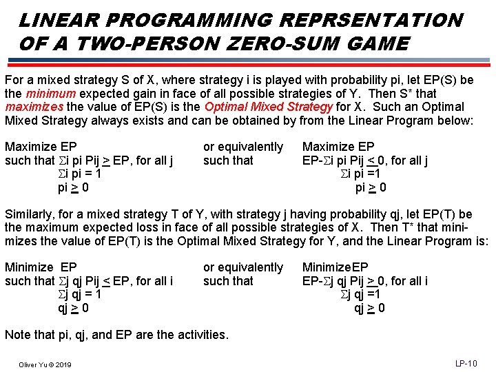
LINEAR PROGRAMMING REPRSENTATION OF A TWO-PERSON ZERO-SUM GAME For a mixed strategy S of X, where strategy i is played with probability pi, let EP(S) be the minimum expected gain in face of all possible strategies of Y. Then S* that maximizes the value of EP(S) is the Optimal Mixed Strategy for X. Such an Optimal Mixed Strategy always exists and can be obtained by from the Linear Program below: Maximize EP such that Si pi Pij > EP, for all j Si pi = 1 pi > 0 or equivalently such that Maximize EP EP-Si pi Pij < 0, for all j Si pi =1 pi > 0 Similarly, for a mixed strategy T of Y, with strategy j having probability qj, let EP(T) be the maximum expected loss in face of all possible strategies of X. Then T* that minimizes the value of EP(T) is the Optimal Mixed Strategy for Y, and the Linear Program is: Minimize EP such that Sj qj Pij < EP, for all i Sj qj = 1 qj > 0 or equivalently such that Minimize. EP EP-Sj qj Pij > 0, for all i Sj qj =1 qj > 0 Note that pi, qj, and EP are the activities. Oliver Yu © 2019 LP-10

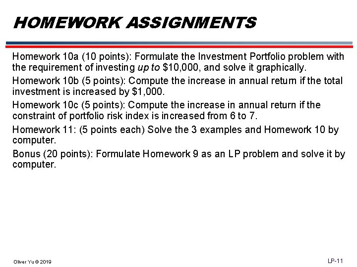
HOMEWORK ASSIGNMENTS Homework 10 a (10 points): Formulate the Investment Portfolio problem with the requirement of investing up to $10, 000, and solve it graphically. Homework 10 b (5 points): Compute the increase in annual return if the total investment is increased by $1, 000. Homework 10 c (5 points): Compute the increase in annual return if the constraint of portfolio risk index is increased from 6 to 7. Homework 11: (5 points each) Solve the 3 examples and Homework 10 by computer. Bonus (20 points): Formulate Homework 9 as an LP problem and solve it by computer. Oliver Yu © 2019 LP-11