Linear Programming Models Graphical and Computer Methods Linear

Linear Programming Models: Graphical and Computer Methods Linear Programming Part 1 Unit 8

Objectives 1. Understand the basic assumptions and properties of linear programming (LP). 2. Use graphical procedures to solve LP problems with only two variables to understand how LP problems are solved. 3. Understand special situations such as redundancy, infeasibility, unboundedness, and alternate optimal solutions in LP problems. 4. Understand how to set up LP problems on a spreadsheet and solve them using Excel’s Solver.

Introduction • Management decisions involve the most effective use of resources • Most widely used modeling technique is linear programming (LP) • Deterministic models

Some Applications • Manufacturing • Factory planning • Refinery planning • Financial Management • Portfolio selection • Human Resources • Scheduling • Transportation • Vehicle routing

Developing a LP Model • Three distinct steps 1. Formulation • mathematical expressions 2. Solution • optimal (or best) solution 3. Interpretation

Key Components • Maximize or minimize some quantity – max profit, min cost • Include restrictions or constraints • Objective and constraints expressed as linear equations (=, ≤, ≥)

LP Characteristics • Feasible Region – • Set of points that satisfies all constraints • Corner Point Property – • Optimal, unique solution must lie at one or more corner points • Optimal Solution – • Corner point with best objective function value

Decision Variables • What we are solving for • Decision variables can be in different units of measurement

The Objective Function • States goal of a problem • maximize profit or minimize cost • Single function

Constraints • Restrictions or limits on our decisions • As many as necessary • Can be independent

Our Action Plan (We will solve the following problems together) • State the decision variables • State the objective function • State the constraints • Sketch the objective function and constraints on graph • Identify the feasible region (all possible solutions) • Identify the optimal (best, profit maximizing in this case) solution.

Guidelines • Recognizing and defining decision variables • Different variables, different units • Use only the decision variables in the model • Difficulties may point to a need for more variables or better definitions

Guidelines • One unit of measurement per expression • Example – wiring time, testing time, units demanded • Constraints are separate • Translate words into expressions

Example – Electrotech Corporation • The Electrotech Corporation manufactures two industrial sized electrical devices: generators and alternators. Both of these products require wiring and testing during the assembly process. Each generator requires 2 hours of wiring and 1 hour of testing and can be sold for a $250 profit. Each alternator requires 3 hours of wiring and 2 hours of testing and can be sold for a $150 profit. There are 260 hours of wiring time and 140 hours of testing time available in the next production period, and Electrotech wants to maximize profit. Formulate an LP model for this problem. Solve graphically.

Cost Minimization – American Auto • American Auto is evaluating its marketing plan for the sedans, SUVs, and trucks the company produces. A TV ad featuring it’s SUV has been developed. The company estimates each showing of this commercial will cost $500, 000 and increase sales of SUVs by 3%, but reduce sales of trucks by 1%, and have no effect on the sales of sedans. The company also has a print ad campaign developed that it can run in various nationally distributed magazines at a cost of $750, 000 per title. It is estimated that each magazine title the ad runs in will increase the sales of sedans, SUVs, and trucks by 2%, 1%, and 4%, respectively. The company desires to increase sales of sedans, SUVs, and trucks by at least 3%, 14%, and 4%, respectively, in the least costly manner. Formulate and graph the LP model for this problem.

Detailed Solutions to Text Problems • The following problems are solved in detail in the text but I’m including them here in case you don’t have the second edition. • There are detailed screen shots of the excel instructions – VERY USEFUL IF YOU CAN’T REMEMBER WHAT WE DID IN CLASS OR NEED A REFERENCE!!!

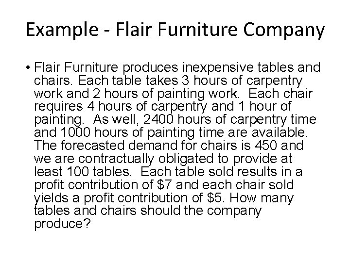
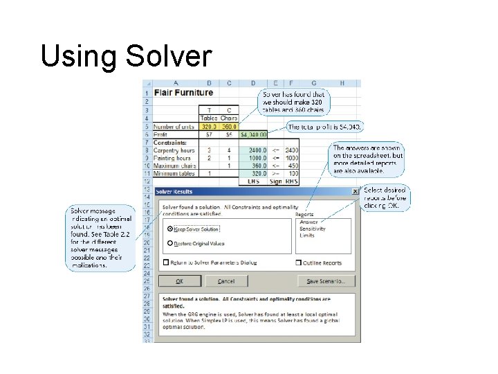
Example - Flair Furniture Company • Flair Furniture produces inexpensive tables and chairs. Each table takes 3 hours of carpentry work and 2 hours of painting work. Each chair requires 4 hours of carpentry and 1 hour of painting. As well, 2400 hours of carpentry time and 1000 hours of painting time are available. The forecasted demand for chairs is 450 and we are contractually obligated to provide at least 100 tables. Each table sold results in a profit contribution of $7 and each chair sold yields a profit contribution of $5. How many tables and chairs should the company produce?

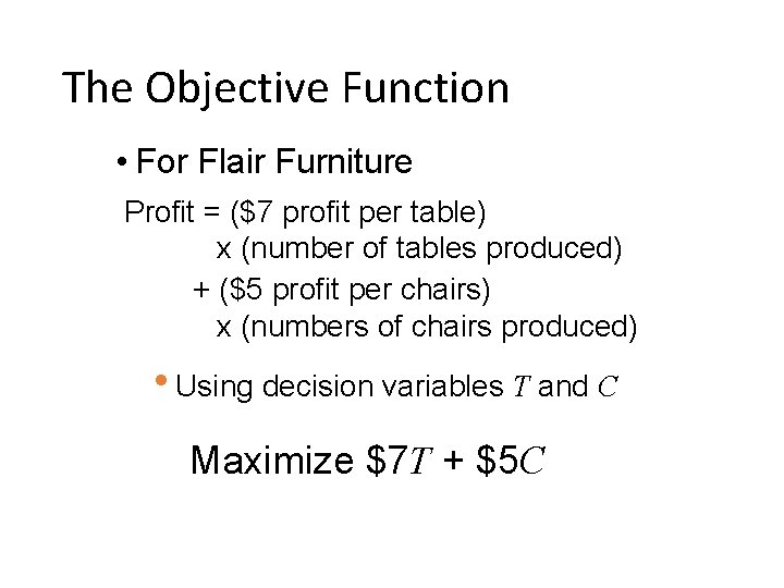
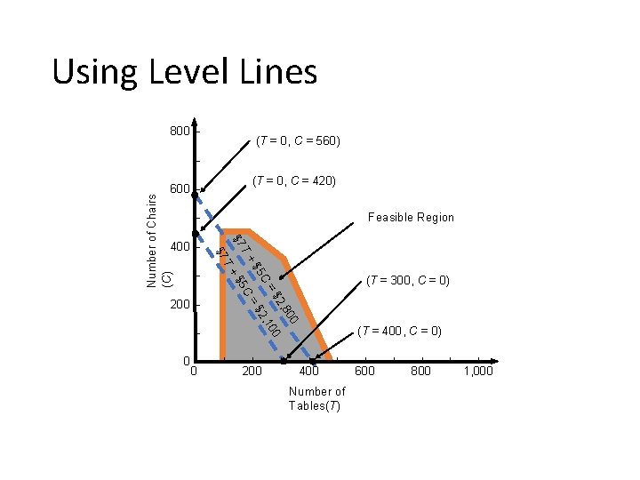
The Objective Function • For Flair Furniture Profit = ($7 profit per table) x (number of tables produced) + ($5 profit per chairs) x (numbers of chairs produced) • Using decision variables T and C Maximize $7 T + $5 C

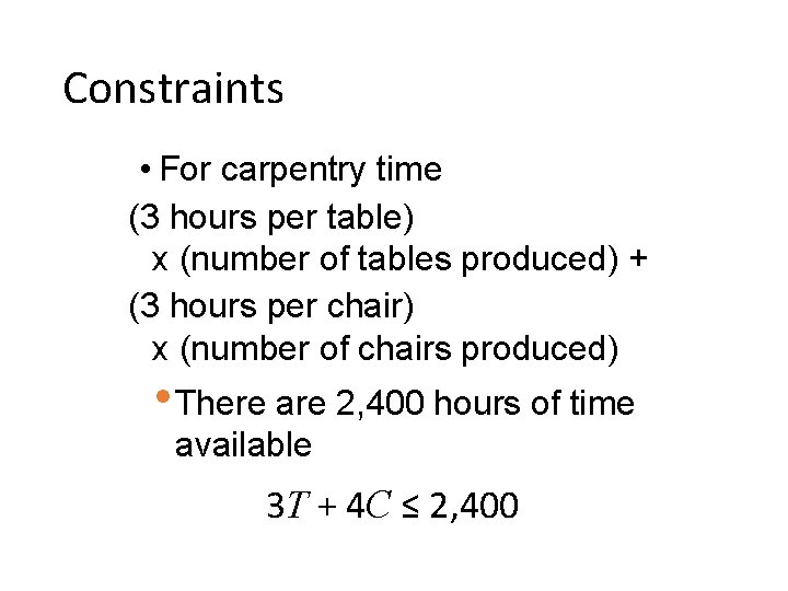
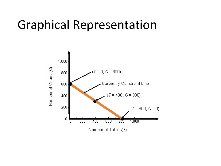
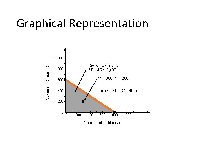
Constraints • For carpentry time (3 hours per table) x (number of tables produced) + (3 hours per chair) x (number of chairs produced) • There are 2, 400 hours of time available 3 T + 4 C ≤ 2, 400

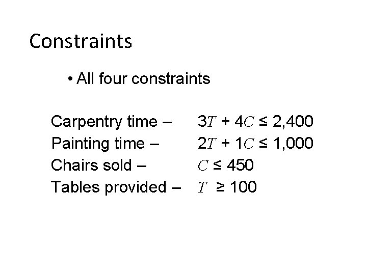
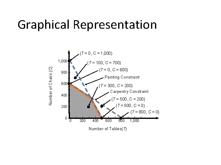
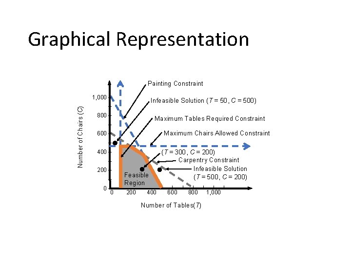
Constraints • All four constraints Carpentry time – Painting time – Chairs sold – Tables provided – 3 T + 4 C ≤ 2, 400 2 T + 1 C ≤ 1, 000 C ≤ 450 T ≥ 100

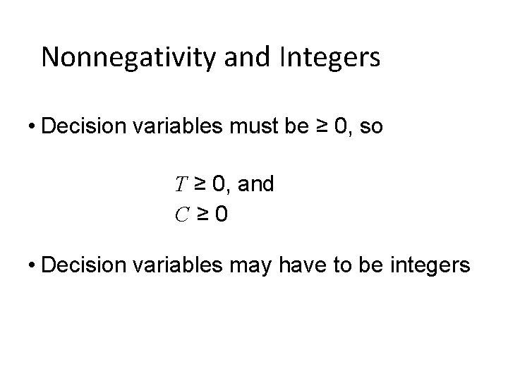
Nonnegativity and Integers • Decision variables must be ≥ 0, so T ≥ 0, and C≥ 0 • Decision variables may have to be integers

Guidelines • Recognizing and defining decision variables • Different variables, different units • Use only the decision variables in the model • Difficulties may point to a need for more variables or better definitions

Guidelines • One unit of measurement per expression • Example – carpentry time, chairs demanded • Constraints are separate • Translate words into expressions

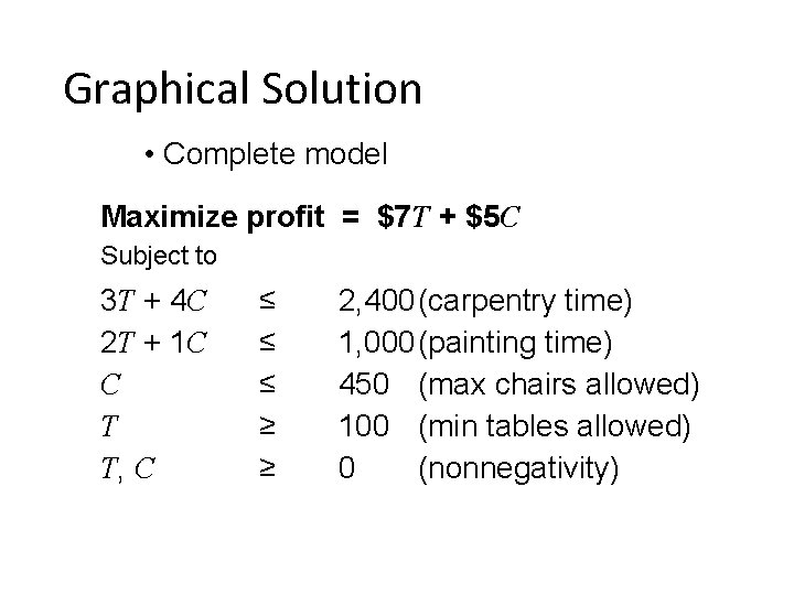
Graphical Solution • Complete model Maximize profit = $7 T + $5 C Subject to 3 T + 4 C 2 T + 1 C C T T, C ≤ ≤ ≤ ≥ ≥ 2, 400(carpentry time) 1, 000(painting time) 450 (max chairs allowed) 100 (min tables allowed) 0 (nonnegativity)

Graphical Representation Number of Chairs (C) 1, 000 – – (T = 0, C = 600) 800 – – Carpentry Constraint Line 600 – – (T = 400, C = 300) 400 – – 200 – (T = 800, C = 0) – 0 –| 0 | | 200 | | 400 | | 600 | | 800 Number of Tables(T) | | 1, 000 |

Graphical Representation Number of Chairs (C) 1, 000 – – Region Satisfying 3 T + 4 C ≤ 2, 400 800 – – (T = 300, C = 200) 600 – – (T = 600, C = 400) 400 – – 200 – – 0 –| 0 | | 200 | | 400 | | 600 | | 800 Number of Tables(T) | | 1, 000 |

Graphical Representation (T = 0, C = 1, 000) Number of Chairs (C) 1, 000 – (T = 100, C = 700) – (T = 0, C = 600) 800 – Painting Constraint – 600 – (T = 300, C = 200) Carpentry Constraint – 400 – – (T = 500, C = 200) 200 – (T = 500, C = 0) (T = 800, C = 0) – 0 –| 0 | | 200 | | 400 | | 600 | | 800 Number of Tables(T) | | 1, 000 |

Graphical Representation Painting Constraint Number of Chairs (C) 1, 000 – Infeasible Solution (T = 50, C = 500) – 800 – Maximum Tables Required Constraint – Maximum Chairs Allowed Constraint 600 – – 400 – (T = 300, C = 200) Carpentry Constraint Infeasible Solution (T = 500, C = 200) – 200 – – 0 –| 0 | Feasible Region | | 200 | 400 | | 600 | | 800 Number of Tables(T) | | 1, 000 |

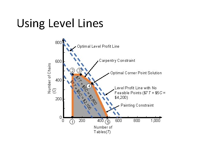
Using Level Lines 800 – (T = 0, C = 560) – (T = 0, C = 420) Feasible Region – T =$ – 0– 0 (T = 300, C = 0) 00 2, 8 00 =$ 2, 1 C $5 200 – 5 C +$ T+ – $7 400 – $7 Number of Chairs (C) 600 – | | 200 | (T = 400, C = 0) | | 400 Number of Tables(T) | 600 | | 800 | | 1, 000

Using Level Lines 800 – Optimal Level Profit Line – Carpentry Constraint – Optimal Corner Point Solution T Level Profit Line with No Feasible Points ($7 T + $5 C = $4, 200) =$ – 0– 0 4 00 2, 8 00 =$ 2, 1 C $5 200 – 5 C +$ T+ – 3 $7 400 – 2 $7 Number of Chairs (C) 600 – | 1 | 200 | Painting Constraint | | | 400 5 600 Number of Tables(T) | | 800 | | 1, 000

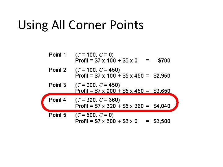
Using All Corner Points Point 1 (T = 100, C = 0) Profit = $7 x 100 + $5 x 0 Point 2 (T = 100, C = 450) Profit = $7 x 100 + $5 x 450 = $2, 950 Point 3 (T = 200, C = 450) Profit = $7 x 200 + $5 x 450 = $3, 650 Point 4 (T = 320, C = 360) Profit = $7 x 320 + $5 x 360 = $4, 040 Point 5 (T = 500, C = 0) Profit = $7 x 500 + $5 x 0 = $700 = $3, 500

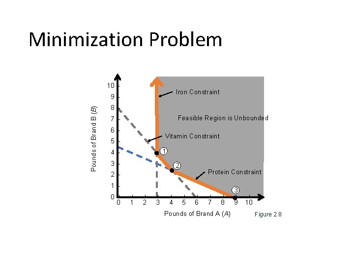
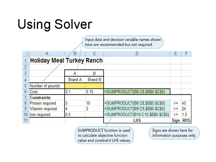
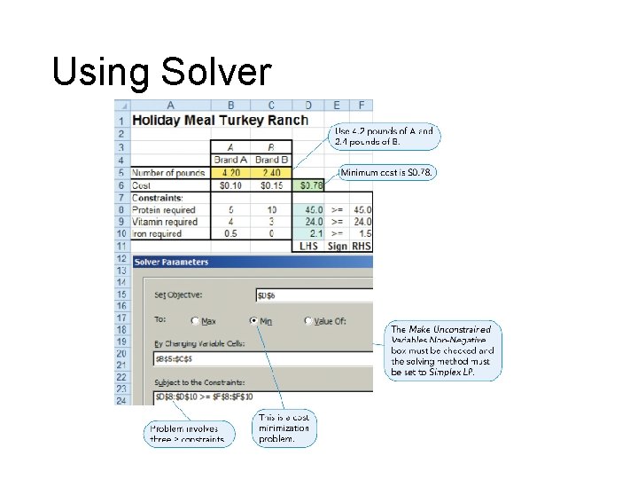
Minimization (Cost) Problem • The Holiday Meal Turkey Ranch has two different brands of turkey feed – brand A and brand B. Each feed contains different quantities of three nutrients (protein, vitamins, and iron) essential for fattening turkeys. Brand A feed costs $0. 10 per lb and brand B costs $0. 15 per lb. The ranch wants to determine the quantity of feed to use to meet the minimum monthly requirements at the lowest cost.

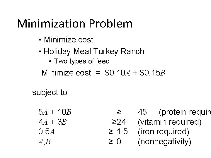
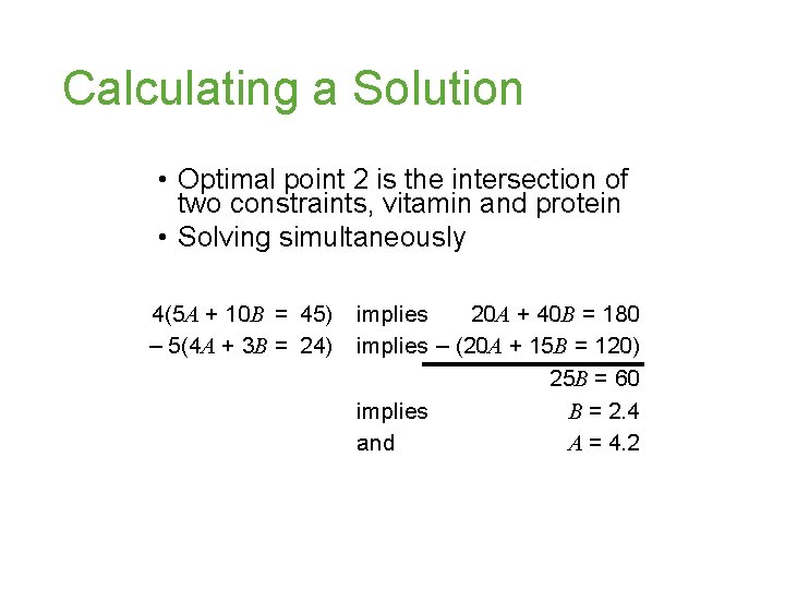
Minimization Problem • Minimize cost • Holiday Meal Turkey Ranch • Two types of feed Minimize cost = $0. 10 A + $0. 15 B subject to 5 A + 10 B 4 A + 3 B 0. 5 A A, B ≥ ≥ 24 ≥ 1. 5 ≥ 0 45 (protein require (vitamin required) (iron required) (nonnegativity)

Minimization Problem 10 – Iron Constraint Pounds of Brand B (B) 9– 8– Feasible Region is Unbounded 7– 6– Vitamin Constraint 5– 1 4– 3– 2 Protein Constraint 2– 1– 0– 0 | 3 | | | | | 1 2 3 4 5 6 7 8 9 10 Pounds of Brand A (A) Figure 2. 8

Calculating a Solution • Optimal point 2 is the intersection of two constraints, vitamin and protein • Solving simultaneously 4(5 A + 10 B = 45) – 5(4 A + 3 B = 24) implies 20 A + 40 B = 180 implies – (20 A + 15 B = 120) 25 B = 60 implies B = 2. 4 and A = 4. 2

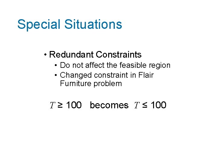
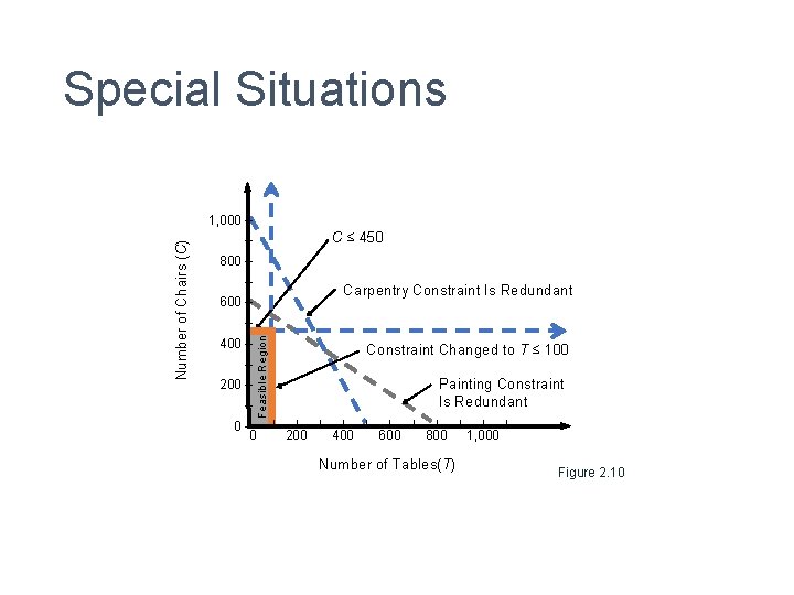
Special Situations • Redundant Constraints • Do not affect the feasible region • Changed constraint in Flair Furniture problem T ≥ 100 becomes T ≤ 100

Special Situations C ≤ 450 – 800 – – Carpentry Constraint Is Redundant 600 – – 400 – – 200 – – Feasible Region Number of Chairs (C) 1, 000 – 0 –| 0 Constraint Changed to T ≤ 100 Painting Constraint Is Redundant | | 200 | | 400 | | 600 | | 800 Number of Tables(T) | | | 1, 000 Figure 2. 10

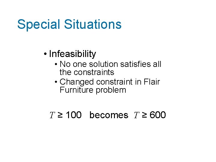
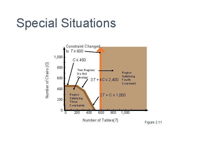
Special Situations • Infeasibility • No one solution satisfies all the constraints • Changed constraint in Flair Furniture problem T ≥ 100 becomes T ≥ 600

Special Situations Constraint Changed to T ≥ 600 Number of Chairs (C) 1, 000 – C ≤ 450 – 800 – Two Regions Do Not Overlap – 600 – Region Satisfying Fourth Constraint 3 T + 4 C ≤ 2, 400 – – 200 – – 0 –| 0 Region Satisfying Three Constraints | | 200 | 2 T + C ≤ 1, 000 | 400 | | 600 | | 800 Number of Tables(T) | | | 1, 000 Figure 2. 11

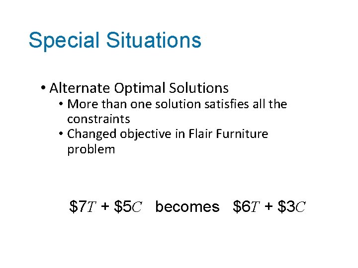
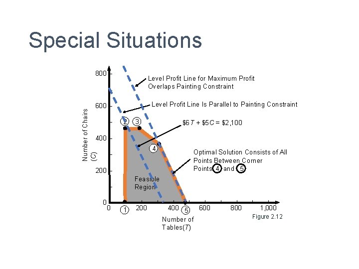
Special Situations • Alternate Optimal Solutions • More than one solution satisfies all the constraints • Changed objective in Flair Furniture problem $7 T + $5 C becomes $6 T + $3 C

Special Situations 800 – Level Profit Line for Maximum Profit Overlaps Painting Constraint – Level Profit Line Is Parallel to Painting Constraint Number of Chairs (C) 600 – – 2 3 $6 T + $5 C = $2, 100 400 – 4 – Optimal Solution Consists of All Points Between Corner Points 4 and 5 200 – Feasible Region – 0– 0 | 1 | 200 | | 400 5 600 Number of Tables(T) | | 800 | | 1, 000 Figure 2. 12

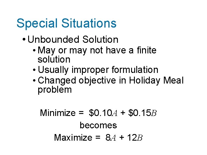
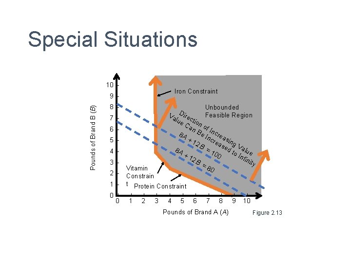
Special Situations • Unbounded Solution • May or may not have a finite solution • Usually improper formulation • Changed objective in Holiday Meal problem Minimize = $0. 10 A + $0. 15 B becomes Maximize = 8 A + 12 B

Special Situations 10 – Iron Constraint Pounds of Brand B (B) 9– 8– Unbounded D i Va rec Feasible Region lue tio Ca n o n B f In cre e 8 A + 1 Incre asin 2 B as g V = 1 ed t alue 8 A o. I 00 +1 nfi 2 B nit y =8 0 7– 6– 5– 4– 3– 2– 1– 0 –| 0 Vitamin Constrain t Protein Constraint | | | | | 1 2 3 4 5 6 7 8 9 10 Pounds of Brand A (A) Figure 2. 13

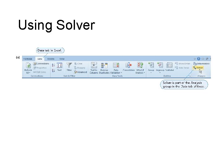
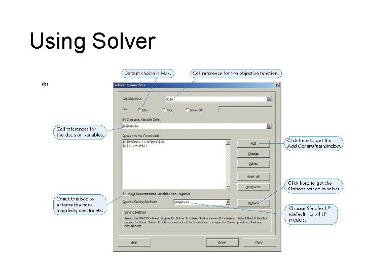
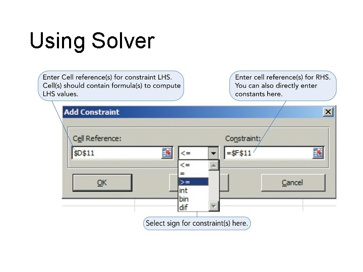
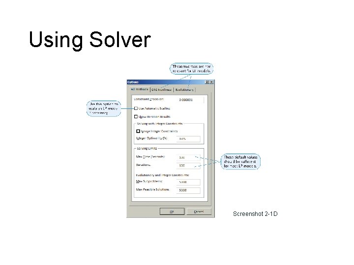
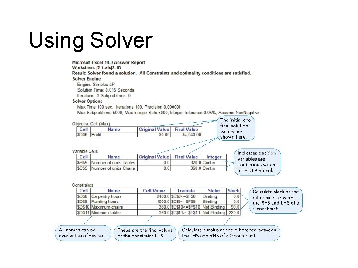
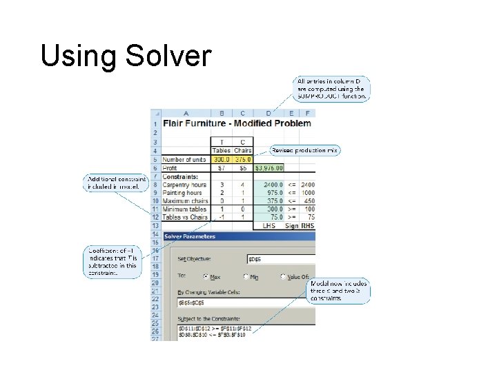
Using Excel’s Solver • Excel’s built-in LP solution tool for LP • Commonly available and easy access • Familiar software

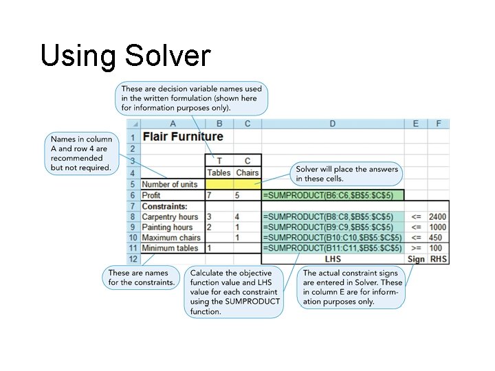
Using Solver

Using Solver

Using Solver

Using Solver

Using Solver Screenshot 2 -1 D

Using Solver

Using Solver

Using Solver

Using Solver

Using Solver