Linear Programming Model Formulation and Graphical Solution Chapter

Linear Programming: Model Formulation and Graphical Solution Chapter 2 Copyright © 2010 Pearson Education, Inc. Publishing as Prentice Hall 2 -1

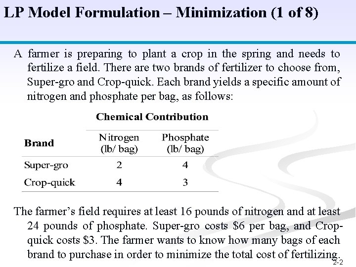
LP Model Formulation – Minimization (1 of 8) A farmer is preparing to plant a crop in the spring and needs to fertilize a field. There are two brands of fertilizer to choose from, Super-gro and Crop-quick. Each brand yields a specific amount of nitrogen and phosphate per bag, as follows: The farmer’s field requires at least 16 pounds of nitrogen and at least 24 pounds of phosphate. Super-gro costs $6 per bag, and Cropquick costs $3. The farmer wants to know how many bags of each brand to purchase in order to minimize the total cost of fertilizing. 2 -2

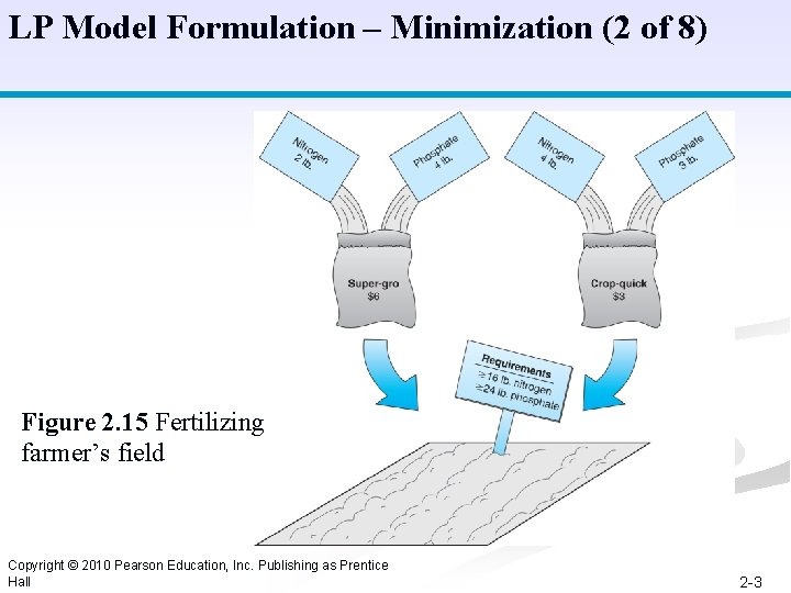
LP Model Formulation – Minimization (2 of 8) Figure 2. 15 Fertilizing farmer’s field Copyright © 2010 Pearson Education, Inc. Publishing as Prentice Hall 2 -3

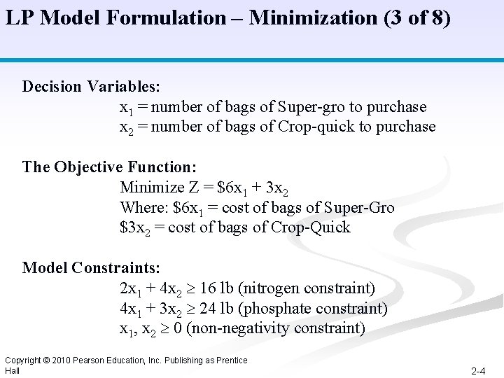
LP Model Formulation – Minimization (3 of 8) Decision Variables: x 1 = number of bags of Super-gro to purchase x 2 = number of bags of Crop-quick to purchase The Objective Function: Minimize Z = $6 x 1 + 3 x 2 Where: $6 x 1 = cost of bags of Super-Gro $3 x 2 = cost of bags of Crop-Quick Model Constraints: 2 x 1 + 4 x 2 16 lb (nitrogen constraint) 4 x 1 + 3 x 2 24 lb (phosphate constraint) x 1, x 2 0 (non-negativity constraint) Copyright © 2010 Pearson Education, Inc. Publishing as Prentice Hall 2 -4

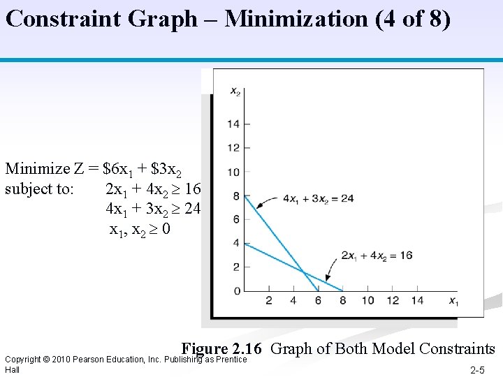
Constraint Graph – Minimization (4 of 8) Minimize Z = $6 x 1 + $3 x 2 subject to: 2 x 1 + 4 x 2 16 4 x 1 + 3 x 2 24 x 1, x 2 0 Figure 2. 16 Graph of Both Model Constraints Copyright © 2010 Pearson Education, Inc. Publishing as Prentice Hall 2 -5

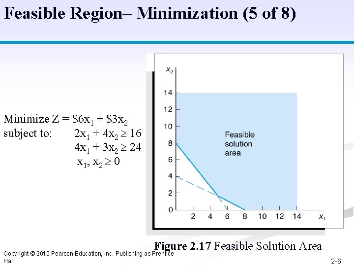
Feasible Region– Minimization (5 of 8) Minimize Z = $6 x 1 + $3 x 2 subject to: 2 x 1 + 4 x 2 16 4 x 1 + 3 x 2 24 x 1, x 2 0 Figure 2. 17 Feasible Solution Area Copyright © 2010 Pearson Education, Inc. Publishing as Prentice Hall 2 -6

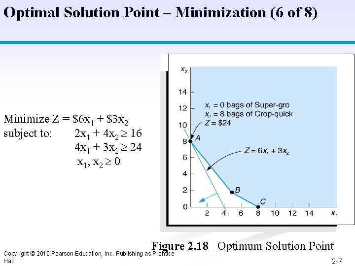
Optimal Solution Point – Minimization (6 of 8) Minimize Z = $6 x 1 + $3 x 2 subject to: 2 x 1 + 4 x 2 16 4 x 1 + 3 x 2 24 x 1, x 2 0 Figure 2. 18 Optimum Solution Point Copyright © 2010 Pearson Education, Inc. Publishing as Prentice Hall 2 -7

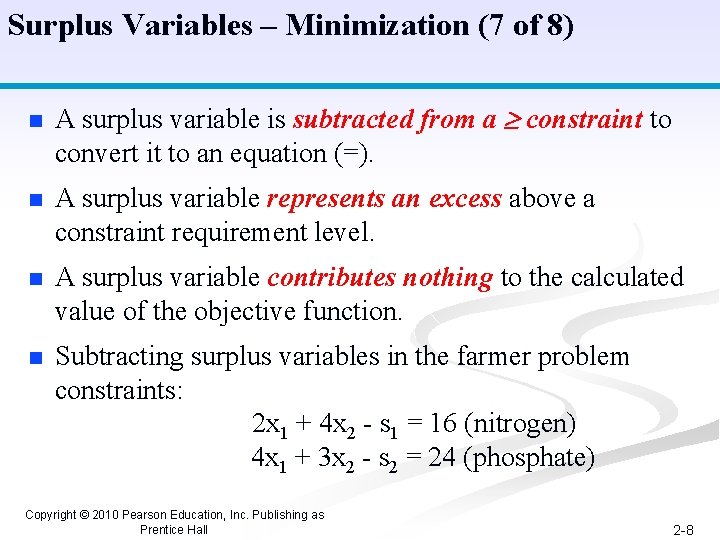
Surplus Variables – Minimization (7 of 8) n A surplus variable is subtracted from a constraint to convert it to an equation (=). n A surplus variable represents an excess above a constraint requirement level. n A surplus variable contributes nothing to the calculated value of the objective function. n Subtracting surplus variables in the farmer problem constraints: 2 x 1 + 4 x 2 - s 1 = 16 (nitrogen) 4 x 1 + 3 x 2 - s 2 = 24 (phosphate) Copyright © 2010 Pearson Education, Inc. Publishing as Prentice Hall 2 -8

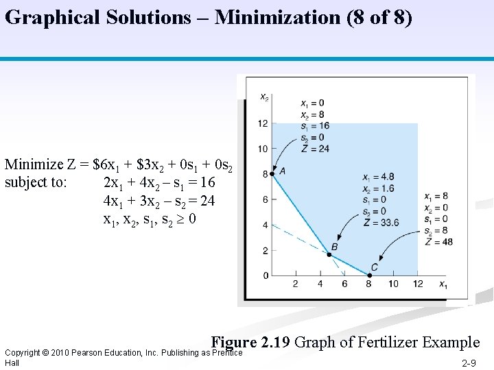
Graphical Solutions – Minimization (8 of 8) Minimize Z = $6 x 1 + $3 x 2 + 0 s 1 + 0 s 2 subject to: 2 x 1 + 4 x 2 – s 1 = 16 4 x 1 + 3 x 2 – s 2 = 24 x 1, x 2, s 1, s 2 0 Figure 2. 19 Graph of Fertilizer Example Copyright © 2010 Pearson Education, Inc. Publishing as Prentice Hall 2 -9

Irregular Types of Linear Programming Problems For some linear programming models, the general rules do not apply. n Special types of problems include those with: § Multiple optimal solutions § Infeasible solutions § Unbounded solutions Copyright © 2010 Pearson Education, Inc. Publishing as Prentice Hall 2 -10

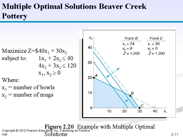
Multiple Optimal Solutions Beaver Creek Pottery Maximize Z=$40 x 1 + 30 x 2 subject to: 1 x 1 + 2 x 2 40 4 x 2 + 3 x 2 120 x 1, x 2 0 Where: x 1 = number of bowls x 2 = number of mugs Figure 2. 20 Example with Multiple Optimal Solutions Copyright © 2010 Pearson Education, Inc. Publishing as Prentice Hall 2 -11

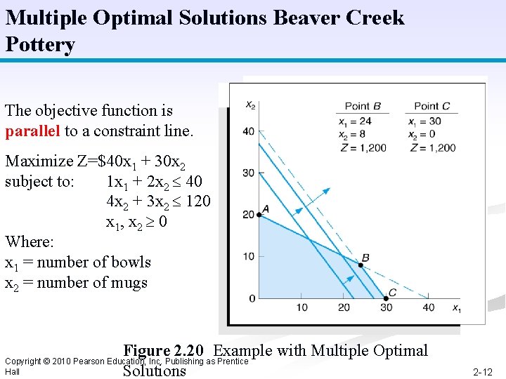
Multiple Optimal Solutions Beaver Creek Pottery The objective function is parallel to a constraint line. Maximize Z=$40 x 1 + 30 x 2 subject to: 1 x 1 + 2 x 2 40 4 x 2 + 3 x 2 120 x 1, x 2 0 Where: x 1 = number of bowls x 2 = number of mugs Figure 2. 20 Example with Multiple Optimal Solutions Copyright © 2010 Pearson Education, Inc. Publishing as Prentice Hall 2 -12

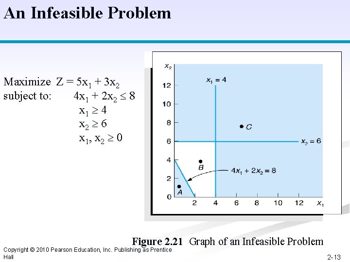
An Infeasible Problem Maximize Z = 5 x 1 + 3 x 2 subject to: 4 x 1 + 2 x 2 8 x 1 4 x 2 6 x 1, x 2 0 Figure 2. 21 Graph of an Infeasible Problem Copyright © 2010 Pearson Education, Inc. Publishing as Prentice Hall 2 -13

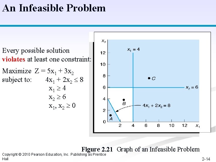
An Infeasible Problem Every possible solution violates at least one constraint: Maximize Z = 5 x 1 + 3 x 2 subject to: 4 x 1 + 2 x 2 8 x 1 4 x 2 6 x 1, x 2 0 Figure 2. 21 Graph of an Infeasible Problem Copyright © 2010 Pearson Education, Inc. Publishing as Prentice Hall 2 -14

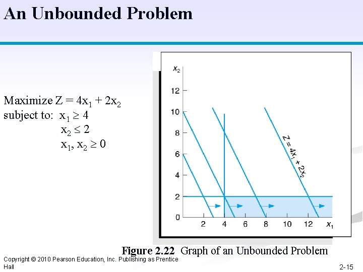
An Unbounded Problem Maximize Z = 4 x 1 + 2 x 2 subject to: x 1 4 x 2 2 x 1, x 2 0 Figure 2. 22 Graph of an Unbounded Problem Copyright © 2010 Pearson Education, Inc. Publishing as Prentice Hall 2 -15

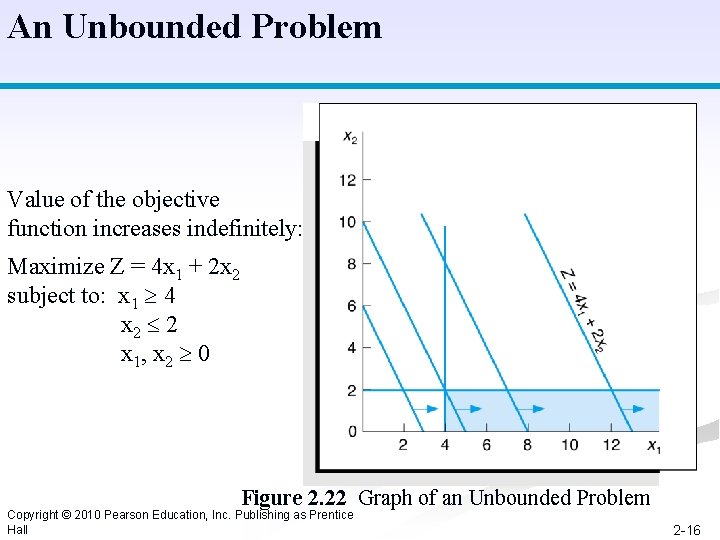
An Unbounded Problem Value of the objective function increases indefinitely: Maximize Z = 4 x 1 + 2 x 2 subject to: x 1 4 x 2 2 x 1, x 2 0 Figure 2. 22 Graph of an Unbounded Problem Copyright © 2010 Pearson Education, Inc. Publishing as Prentice Hall 2 -16

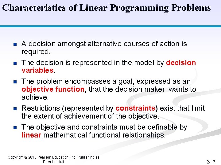
Characteristics of Linear Programming Problems n n n A decision amongst alternative courses of action is required. The decision is represented in the model by decision variables. The problem encompasses a goal, expressed as an objective function, that the decision maker wants to achieve. Restrictions (represented by constraints) exist that limit the extent of achievement of the objective. The objective and constraints must be definable by linear mathematical functional relationships. Copyright © 2010 Pearson Education, Inc. Publishing as Prentice Hall 2 -17

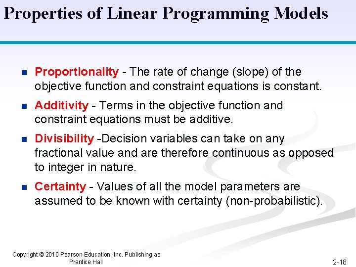
Properties of Linear Programming Models n Proportionality - The rate of change (slope) of the objective function and constraint equations is constant. n Additivity - Terms in the objective function and constraint equations must be additive. n Divisibility -Decision variables can take on any fractional value and are therefore continuous as opposed to integer in nature. n Certainty - Values of all the model parameters are assumed to be known with certainty (non-probabilistic). Copyright © 2010 Pearson Education, Inc. Publishing as Prentice Hall 2 -18

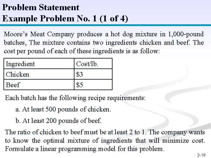
Problem Statement Example Problem No. 1 (1 of 4) Moore’s Meat Company produces a hot dog mixture in 1, 000 -pound batches, The mixture contains two ingredients chicken and beef. The cost per pound of each of these ingredients is as follow: Ingredient Chicken Beef Cost/lb. $3 $5 Each batch has the following recipe requirements: a. At least 500 pounds of chicken. b. At least 200 pounds of beef. The ratio of chicken to beef must be at least 2 to 1. The company wants to know the optimal mixture of ingredients that will minimize cost. Formulate a linear programming model for this problem. 2 -19

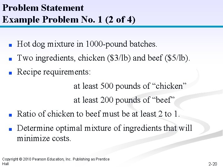
Problem Statement Example Problem No. 1 (2 of 4) ■ Hot dog mixture in 1000 -pound batches. ■ Two ingredients, chicken ($3/lb) and beef ($5/lb). ■ Recipe requirements: at least 500 pounds of “chicken” at least 200 pounds of “beef” ■ Ratio of chicken to beef must be at least 2 to 1. ■ Determine optimal mixture of ingredients that will minimize costs. Copyright © 2010 Pearson Education, Inc. Publishing as Prentice Hall 2 -20

Solution Example Problem No. 1 (3 of 4) 2 -21

Solution Example Problem No. 1 (4 of 4) 2 -22

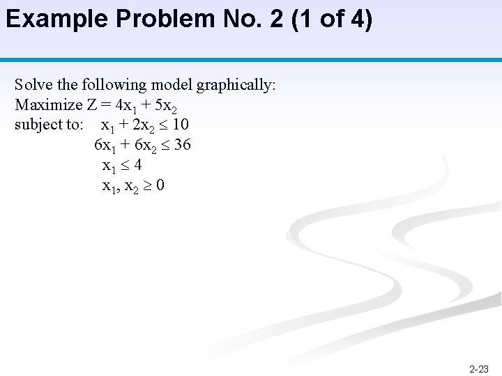
Example Problem No. 2 (1 of 4) Solve the following model graphically: Maximize Z = 4 x 1 + 5 x 2 subject to: x 1 + 2 x 2 10 6 x 1 + 6 x 2 36 x 1 4 x 1, x 2 0 2 -23

Example Problem No. 2 (2 of 4) 2 -24

Example Problem No. 2 (3 of 4) 2 -25

Example Problem No. 2 (4 of 4) 2 -26