Linear Programming LP George Dantzig 1947 1 1

Linear Programming (LP) 線性規劃 - George Dantzig, 1947 1

[1] LP Formulation (a) Decision Variables : All the decision variables are non-negative. (b) Objective Function : Min or Max (c) Constraints s. t. : subject to 2

[2] Example A company has three plants, Plant 1, Plant 2, Plant 3. Because of declining earnings, top management has decided to revamp the company’s product line. Product 1: It requires some of production capacity in Plants 1 and 3. Product 2: It needs Plants 2 and 3. 3

The marketing division has concluded that the company could sell as much as could be produced by these plants. However, because both products would be competing for the same production capacity in Plant 3, it is not clear which mix of the two products would be most profitable. 4

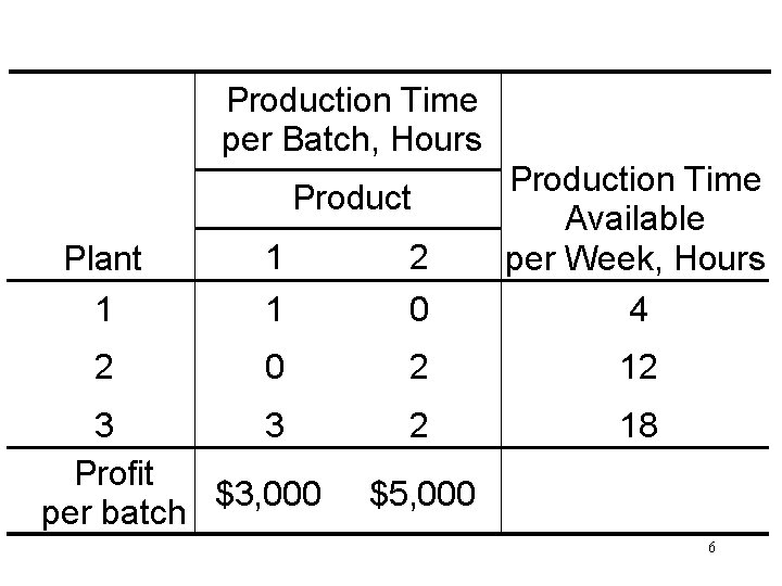
The data needed to be gathered: 1. Number of hours of production time available per week in each plant for these new products. (The available capacity for the new products is quite limited. ) 2. Production time used in each plant for each batch to yield each new product. 3. There is a profit per batch from a new product. 5

Production Time per Batch, Hours Plant 1 1 1 2 0 Production Time Available per Week, Hours 4 2 0 2 12 2 18 Product 3 3 Profit $3, 000 per batch $5, 000 6

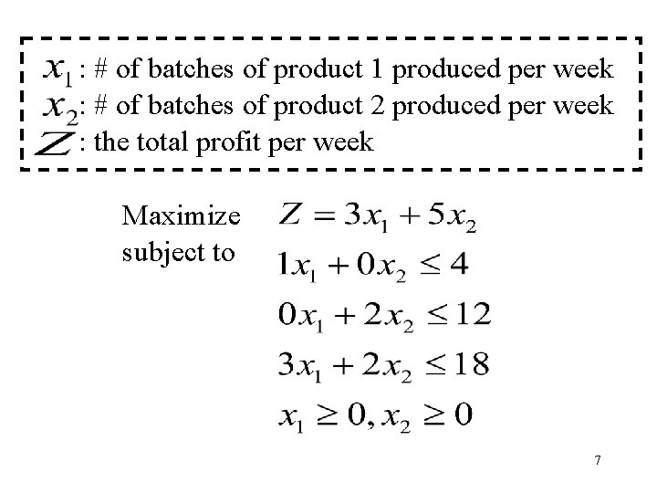
: # of batches of product 1 produced per week : # of batches of product 2 produced per week : the total profit per week Maximize subject to 7

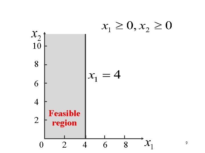
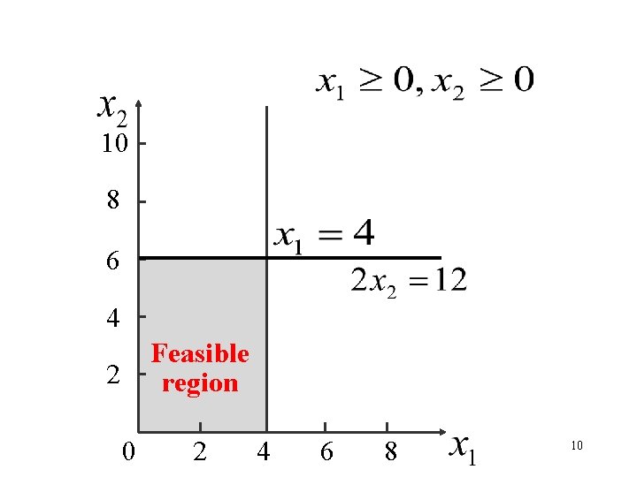
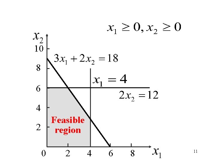
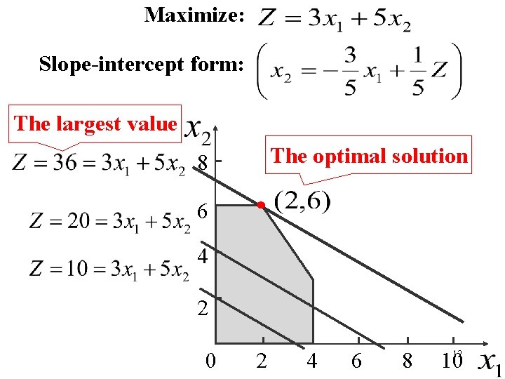
[3] Graphical Solution (only for 2 -variable cases) 10 8 6 4 Feasible region 2 0 2 4 6 8 8

10 8 6 4 Feasible region 2 0 2 4 6 8 9

10 8 6 4 Feasible region 2 0 2 4 6 8 10

10 8 6 4 Feasible region 2 0 2 4 6 8 11

Maximize: Slope-intercept form: The largest value The optimal solution 8 6 4 2 0 2 4 6 8 1012

[4] Standard Form of LP Model Max s. t. 13

[5] Other Forms The other LP forms are the following: 1. Minimizing the objective function: Minimize 2. Greater-than-or-equal-to constraints: 14

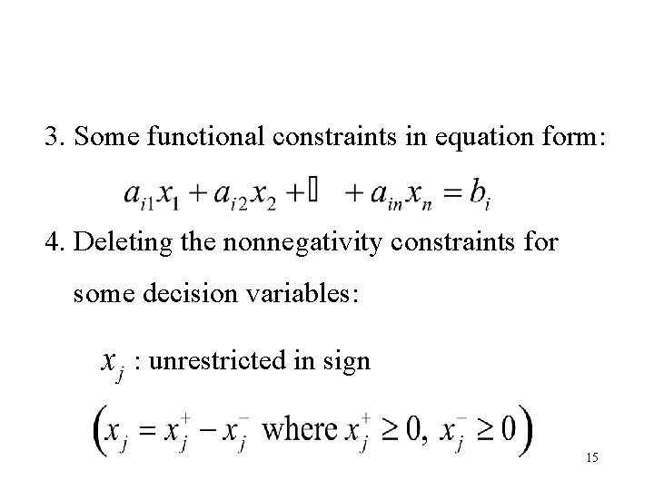
3. Some functional constraints in equation form: 4. Deleting the nonnegativity constraints for some decision variables: : unrestricted in sign 15

[6] Key Terminology (a) A feasible solution is a solution for which all constraints are satisfied (b) An infeasible solution is a solution for which at least one constraint is violated (c) A feasible region is a collection of all feasible solutions 16

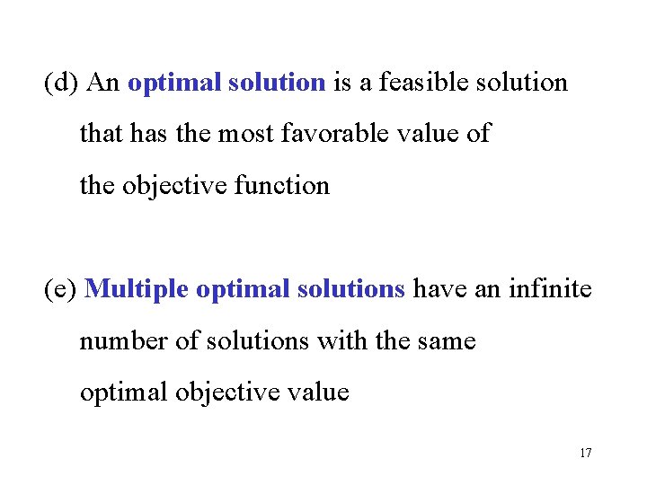
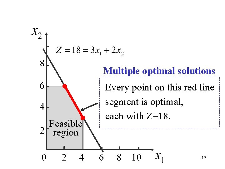
(d) An optimal solution is a feasible solution that has the most favorable value of the objective function (e) Multiple optimal solutions have an infinite number of solutions with the same optimal objective value 17

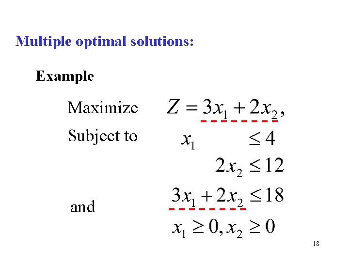
Multiple optimal solutions: Example Maximize Subject to and 18

8 Multiple optimal solutions 6 Every point on this red line segment is optimal, each with Z=18. 4 Feasible 2 region 0 2 4 6 8 10 19

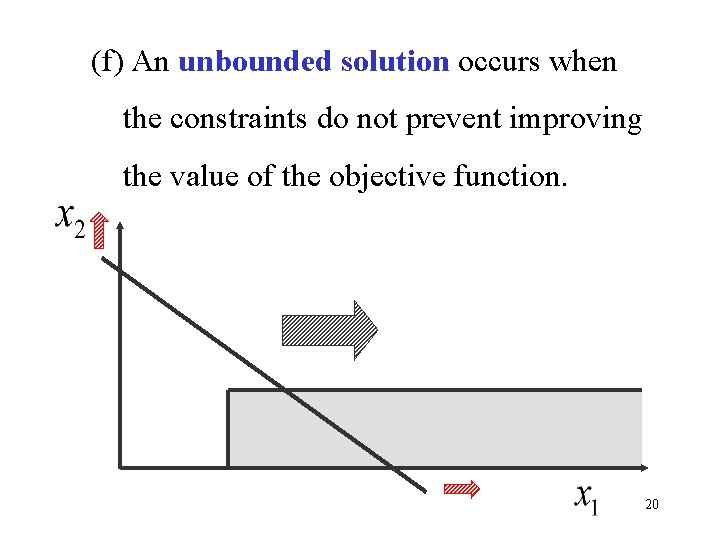
(f) An unbounded solution occurs when the constraints do not prevent improving the value of the objective function. 20

[7] Case Study The Socorro Agriculture Co. is a group of three farming communities. Overall planning for this group is done in its Coordinating Technical Office. This office currently is planning agricultural production for the coming year. 21

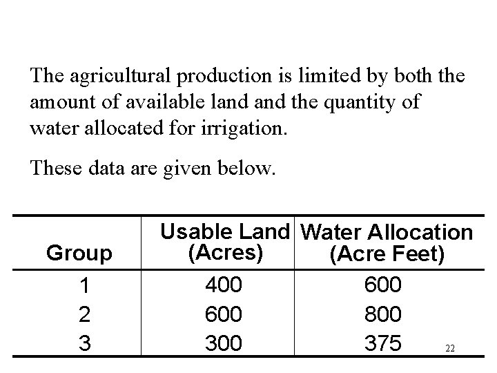
The agricultural production is limited by both the amount of available land the quantity of water allocated for irrigation. These data are given below. Group 1 2 3 Usable Land Water Allocation (Acres) (Acre Feet) 400 600 800 375 22

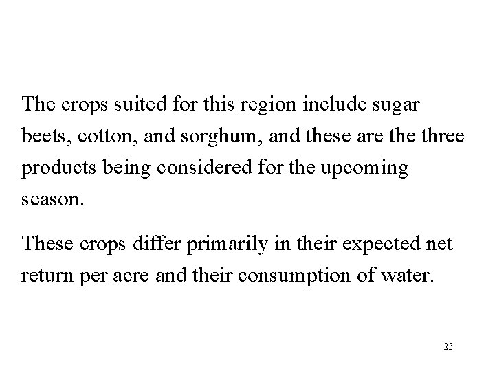
The crops suited for this region include sugar beets, cotton, and sorghum, and these are three products being considered for the upcoming season. These crops differ primarily in their expected net return per acre and their consumption of water. 23

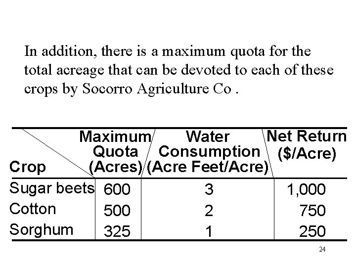
In addition, there is a maximum quota for the total acreage that can be devoted to each of these crops by Socorro Agriculture Co. Net Return Maximum Water Quota Consumption ($/Acre) (Acres) (Acre Feet/Acre) Crop Sugar beets 600 3 1, 000 Cotton 500 2 750 Sorghum 325 1 250 24

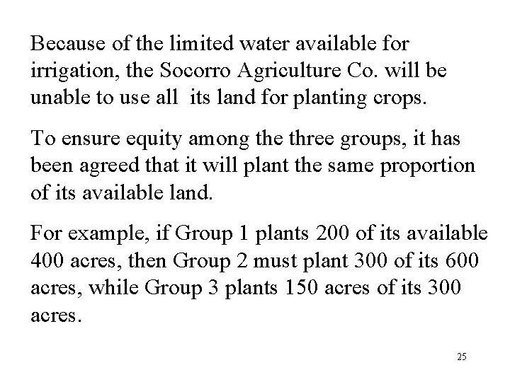
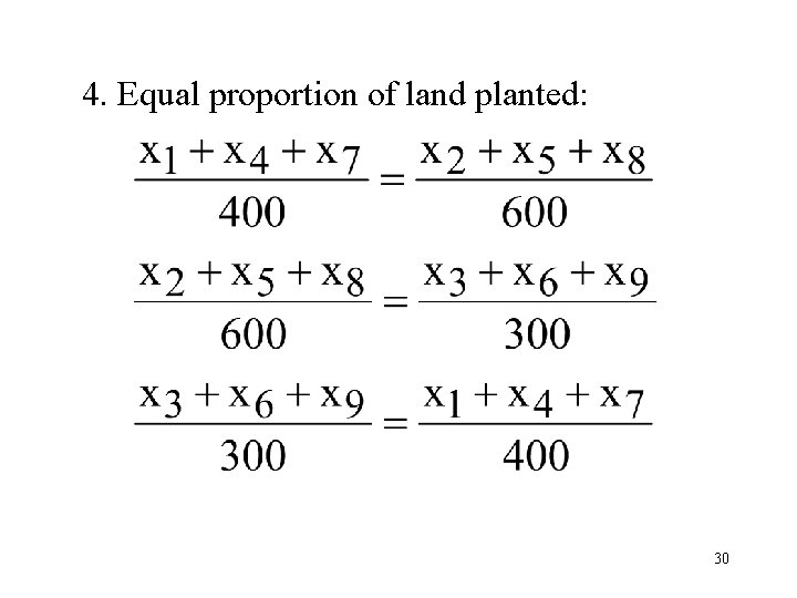
Because of the limited water available for irrigation, the Socorro Agriculture Co. will be unable to use all its land for planting crops. To ensure equity among the three groups, it has been agreed that it will plant the same proportion of its available land. For example, if Group 1 plants 200 of its available 400 acres, then Group 2 must plant 300 of its 600 acres, while Group 3 plants 150 acres of its 300 acres. 25

The job facing the Coordinating Technical Office is to plan how many acres to devote to each crop while satisfying the given restrictions. The objective is to maximize the total net return as a whole. 26

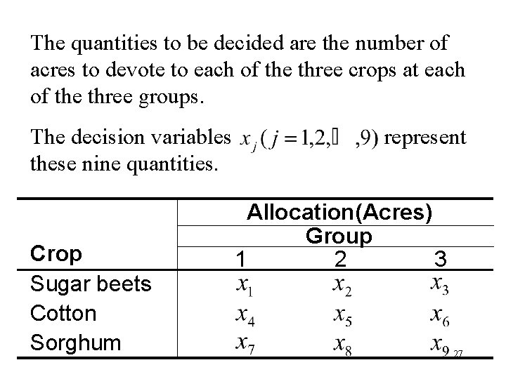
The quantities to be decided are the number of acres to devote to each of the three crops at each of the three groups. The decision variables these nine quantities. Crop Sugar beets Cotton Sorghum represent Allocation(Acres) Group 1 2 3 27

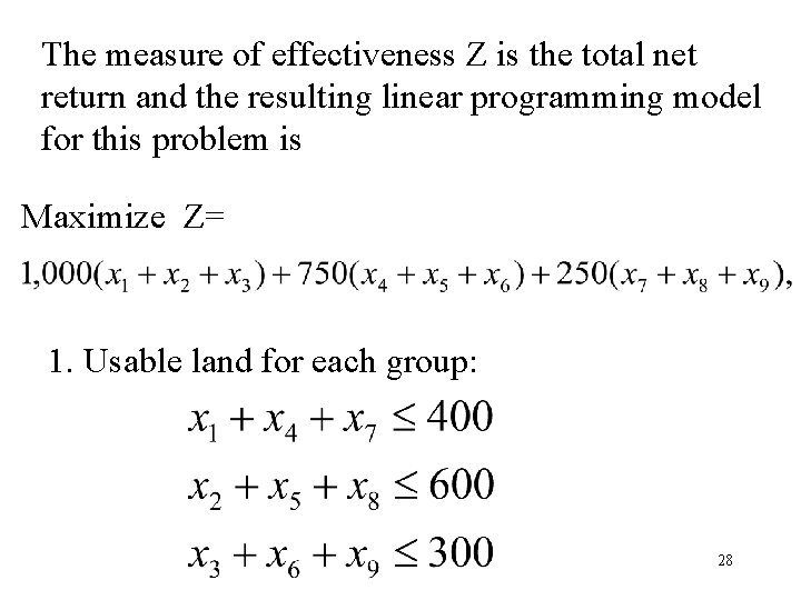
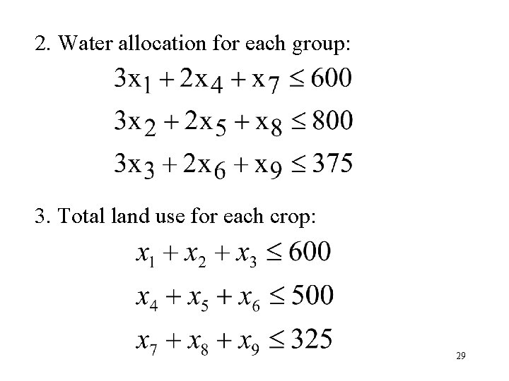
The measure of effectiveness Z is the total net return and the resulting linear programming model for this problem is Maximize Z= 1. Usable land for each group: 28

2. Water allocation for each group: 3. Total land use for each crop: 29

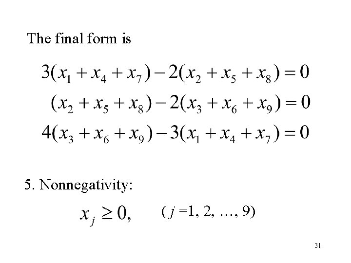
4. Equal proportion of land planted: 30

The final form is 5. Nonnegativity: ( j =1, 2, …, 9) 31

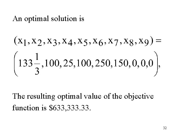
An optimal solution is The resulting optimal value of the objective function is $633, 333. 32

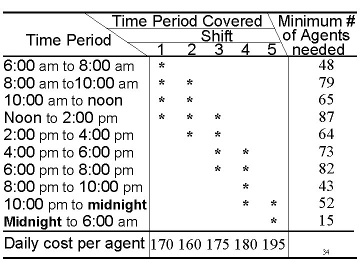
[8] Case Study - Personal Scheduling UNION AIRWAYS needs to hire additional customer service agents. Management recognizes the need for cost control while also consistently providing a satisfactory level of service to customers. Based on the new schedule of flights, an analysis has been made of the minimum number of customer service agents that need to be on duty at different times of the day to provide a satisfactory level of service. 33

Time Period Covered Minimum # of Agents Shift Time Period 1 2 3 4 5 needed 48 6: 00 am to 8: 00 am * 79 8: 00 am to 10: 00 am * * 65 10: 00 am to noon * * 87 Noon to 2: 00 pm * * * 64 2: 00 pm to 4: 00 pm * * 73 4: 00 pm to 6: 00 pm * * 82 6: 00 pm to 8: 00 pm * * 43 8: 00 pm to 10: 00 pm * 52 10: 00 pm to midnight * * 15 Midnight to 6: 00 am * Daily cost per agent 170 160 175 180 195 34

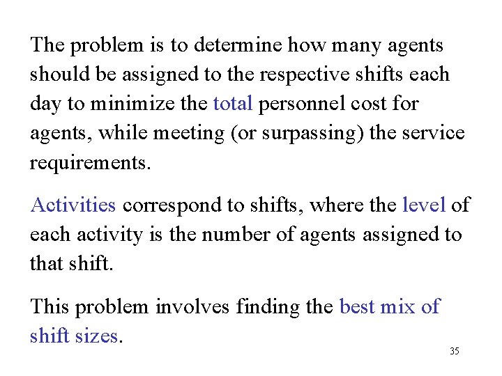
The problem is to determine how many agents should be assigned to the respective shifts each day to minimize the total personnel cost for agents, while meeting (or surpassing) the service requirements. Activities correspond to shifts, where the level of each activity is the number of agents assigned to that shift. This problem involves finding the best mix of shift sizes. 35

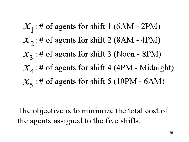
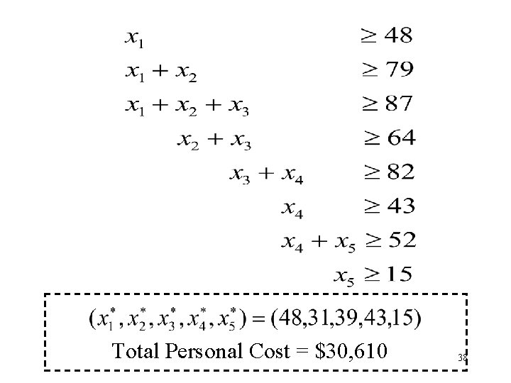
: # of agents for shift 1 (6 AM - 2 PM) : # of agents for shift 2 (8 AM - 4 PM) : # of agents for shift 3 (Noon - 8 PM) : # of agents for shift 4 (4 PM - Midnight) : # of agents for shift 5 (10 PM - 6 AM) The objective is to minimize the total cost of the agents assigned to the five shifts. 36

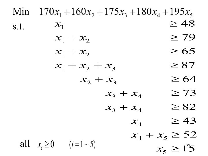
Min s. t. all 37

Total Personal Cost = $30, 610 38

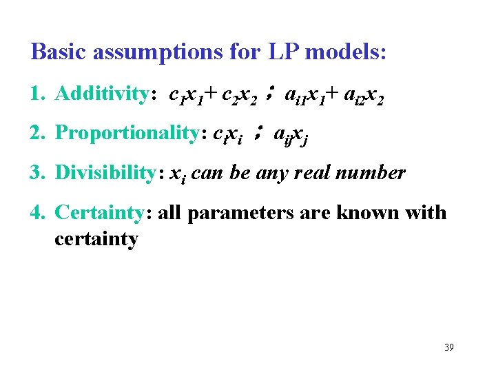
Basic assumptions for LP models: 1. Additivity: c 1 x 1+ c 2 x 2； ai 1 x 1+ ai 2 x 2 2. Proportionality: cixi ； aijxj 3. Divisibility: xi can be any real number 4. Certainty: all parameters are known with certainty 39

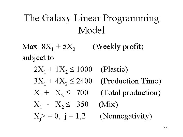
Other Examples • Galaxy manufactures two toy doll models: – Space Ray. – Zapper. • Resources are limited to – 1000 pounds of special plastic. – 40 hours of production time per week. 40

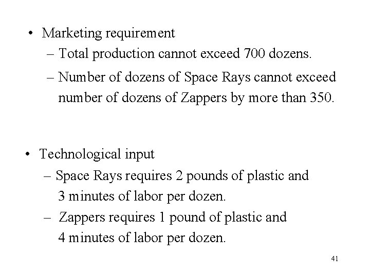
• Marketing requirement – Total production cannot exceed 700 dozens. – Number of dozens of Space Rays cannot exceed number of dozens of Zappers by more than 350. • Technological input – Space Rays requires 2 pounds of plastic and 3 minutes of labor per dozen. – Zappers requires 1 pound of plastic and 4 minutes of labor per dozen. 41

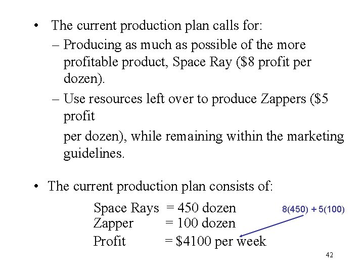
• The current production plan calls for: – Producing as much as possible of the more profitable product, Space Ray ($8 profit per dozen). – Use resources left over to produce Zappers ($5 profit per dozen), while remaining within the marketing guidelines. • The current production plan consists of: Space Rays = 450 dozen Zapper = 100 dozen Profit = $4100 per week 8(450) + 5(100) 42

Management is seeking a production schedule that will increase the company’s profit. 43

A linear programming model can provide an insight and an intelligent solution to this proble 44

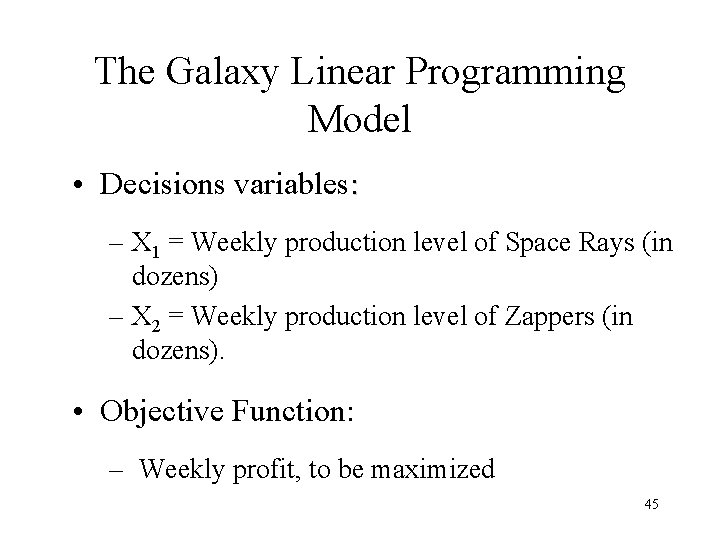
The Galaxy Linear Programming Model • Decisions variables: – X 1 = Weekly production level of Space Rays (in dozens) – X 2 = Weekly production level of Zappers (in dozens). • Objective Function: – Weekly profit, to be maximized 45

The Galaxy Linear Programming Model Max 8 X 1 + 5 X 2 (Weekly profit) subject to 2 X 1 + 1 X 2 £ 1000 (Plastic) 3 X 1 + 4 X 2 £ 2400 (Production Time) X 1 + X 2 £ 700 (Total production) X 1 - X 2 £ 350 (Mix) Xj> = 0, j = 1, 2 (Nonnegativity) 46