Linear Programming from the companion CD Chapter 2

Linear Programming from the companion CD - Chapter 2 of the book: Balakrishnan, Render, and Stair, “Managerial Decision Modeling with Spreadsheets”, 2 nd ed. , Prentice-Hall, 2007 http: //www. stmartin. edu/ Rev. 2. 15 by M. Miccio on January 28, 2014 © 2007 Pearson Education

Introduction to Linear Programming • A Linear Programming (LP) model seeks to maximize or minimize a linear function, subject to a set of linear constraints. • The linear model consists of the following components: – a set of decision variables. – an objective function. – a set of constraints. from the companion CD of the book: Lawrence and Pasternack, “Applied Management Science: Modeling, Spreadsheet Analysis, and Communication for Decision Making”, 2 nd Edition, 2

Introduction to Linear Programming The Importance of Linear Programming – Many real world problems lend themselves to linear programming modeling. – Many real world problems can be approximated by linear models. – There are well-known successful applications in: • Manufacturing • Marketing • Finance (investment) • Advertising • Agriculture from the companion CD of the book: Lawrence and Pasternack, “Applied Management Science: Modeling, Spreadsheet Analysis, and Communication for Decision Making”, 2 nd Edition, 3

Introduction to Linear Programming The Importance of Linear Programming – There are efficient solution techniques that solve linear programming models. – The output generated from linear programming packages provides useful “what if” analysis. from the companion CD of the book: Lawrence and Pasternack, “Applied Management Science: Modeling, Spreadsheet Analysis, and Communication for Decision Making”, 2 nd Edition, 4

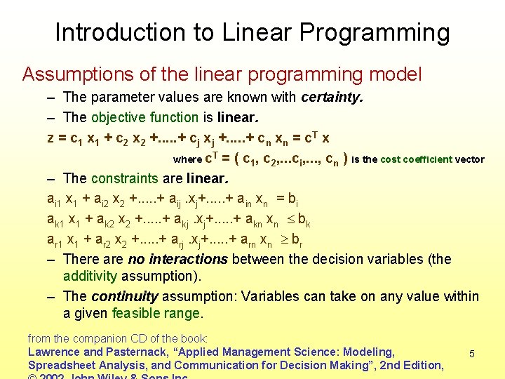
Introduction to Linear Programming Assumptions of the linear programming model – The parameter values are known with certainty. – The objective function is linear. z = c 1 x 1 + c 2 x 2 +. . . + cj xj +. . . + cn xn = c. T x where c. T = ( c 1, c 2, . . . ci, . . . , cn ) is the cost coefficient vector – The constraints are linear. ai 1 x 1 + ai 2 x 2 +. . . + aij. xj+. . . + ain xn = bi ak 1 x 1 + ak 2 x 2 +. . . + akj. xj+. . . + akn xn bk ar 1 x 1 + ar 2 x 2 +. . . + arj. xj+. . . + arn xn br – There are no interactions between the decision variables (the additivity assumption). – The continuity assumption: Variables can take on any value within a given feasible range. from the companion CD of the book: Lawrence and Pasternack, “Applied Management Science: Modeling, Spreadsheet Analysis, and Communication for Decision Making”, 2 nd Edition, 5

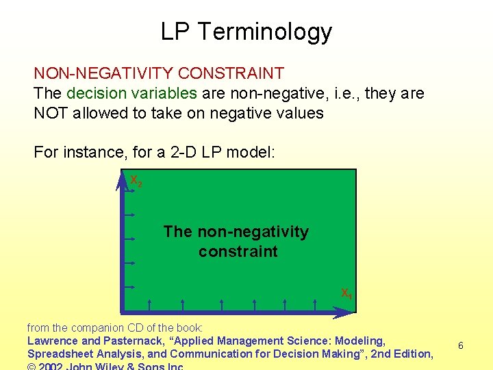
LP Terminology NON-NEGATIVITY CONSTRAINT The decision variables are non-negative, i. e. , they are NOT allowed to take on negative values For instance, for a 2 -D LP model: X 2 The non-negativity constraint X 1 from the companion CD of the book: Lawrence and Pasternack, “Applied Management Science: Modeling, Spreadsheet Analysis, and Communication for Decision Making”, 2 nd Edition, 6

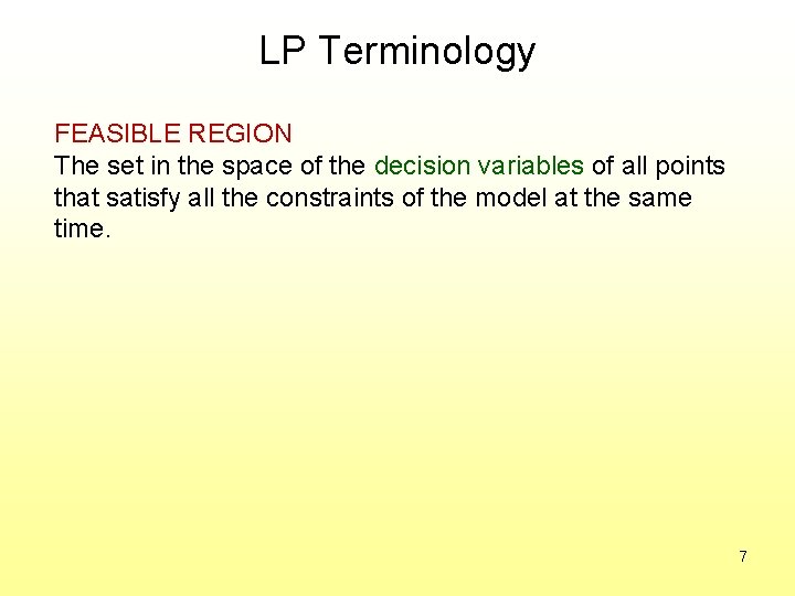
LP Terminology FEASIBLE REGION The set in the space of the decision variables of all points that satisfy all the constraints of the model at the same time. 7

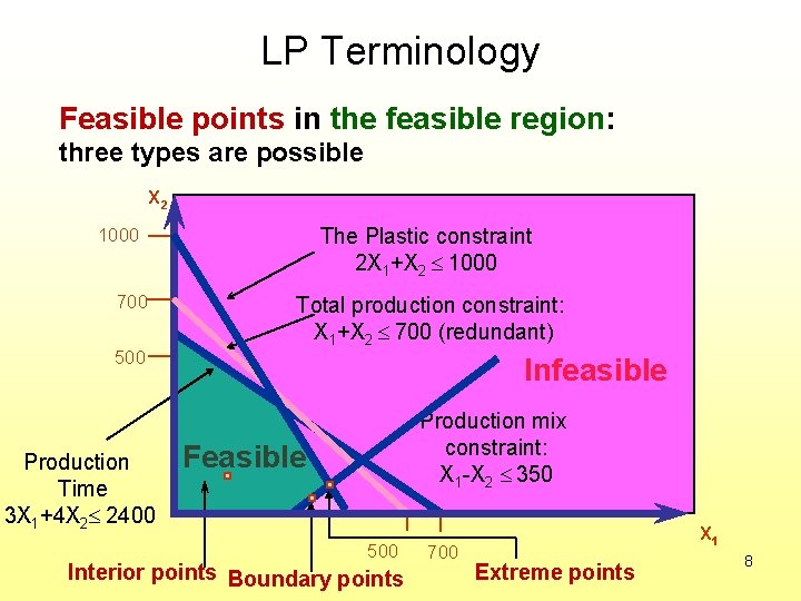
LP Terminology Feasible points in the feasible region: three types are possible X 2 The Plastic constraint 2 X 1+X 2 1000 700 500 Production Time 3 X 1+4 X 2 2400 Total production constraint: X 1+X 2 700 (redundant) Infeasible Production mix constraint: X 1 -X 2 350 Feasible 500 Interior points Boundary points 700 X 1 Extreme points 8

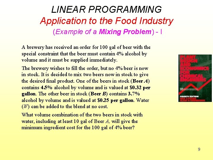
LINEAR PROGRAMMING Application to the Food Industry (Example of a Mixing Problem) - I A brewery has received an order for 100 gal of beer with the special constraint that the beer must contain 4% alcohol by volume and it must be supplied immediately. The brewery wishes to fill the order, but no 4% beer is now in stock. It is decided to mix two beers now in stock to give the desired final product. One of the beers in stock (Beer A) contains 4. 5% alcohol by volume and is valued at $0. 32 per gallon. The other beer in stock (Beer B) contains 3. 7% alcohol by volume and is valued at $0. 25 per gallon. Water (W) can be added to the blend at no cost. What volume combination of the two beers in stock with water, including at least 10 gal of Beer A, will give the minimum ingredient cost for the 100 gal of 4% beer? 9

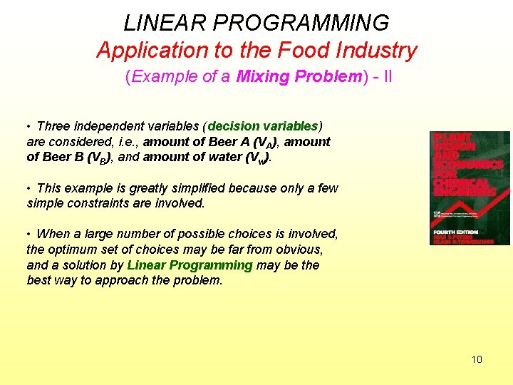
LINEAR PROGRAMMING Application to the Food Industry (Example of a Mixing Problem) - II • Three independent variables (decision variables) are considered, i. e. , amount of Beer A (VA), amount of Beer B (VB), and amount of water (Vw). • This example is greatly simplified because only a few simple constraints are involved. • When a large number of possible choices is involved, the optimum set of choices may be far from obvious, and a solution by Linear Programming may be the best way to approach the problem. 10

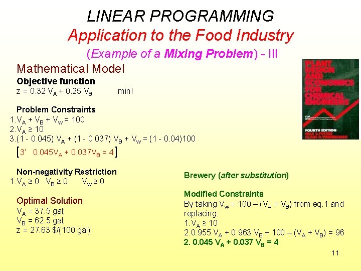
LINEAR PROGRAMMING Application to the Food Industry (Example of a Mixing Problem) - III Mathematical Model Objective function z = 0. 32 VA + 0. 25 VB min! Problem Constraints 1. VA + VB + Vw = 100 2. VA ≥ 10 3. (1 - 0. 045) VA + (1 - 0. 037) VB + Vw = (1 - 0. 04)100 [3’ 0. 045 VA + 0. 037 VB = 4] Non-negativity Restriction 1. VA ≥ 0 VB ≥ 0 Vw ≥ 0 Optimal Solution VA = 37. 5 gal; VB = 62. 5 gal; z = 27. 63 $/(100 gal) Brewery (after substitution) Modified Constraints By taking Vw = 100 – (VA + VB) from eq. 1 and replacing: 1. VA ≥ 10 2. 0. 955 VA + 0. 963 VB + 100 – (VA + VB) = 96 2. 0. 045 VA + 0. 037 VB = 4 11

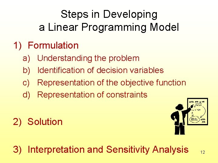
Steps in Developing a Linear Programming Model 1) Formulation a) b) c) d) Understanding the problem Identification of decision variables Representation of the objective function Representation of constraints 2) Solution 3) Interpretation and Sensitivity Analysis 12

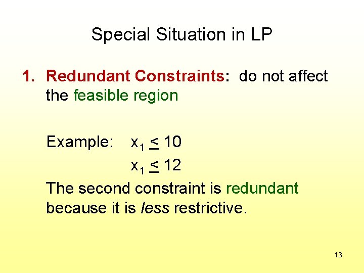
Special Situation in LP 1. Redundant Constraints: do not affect the feasible region Example: x 1 < 10 x 1 < 12 The second constraint is redundant because it is less restrictive. 13

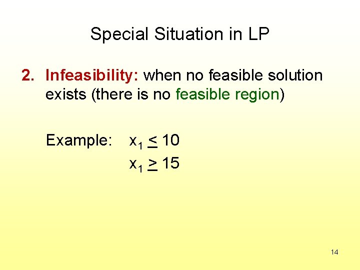
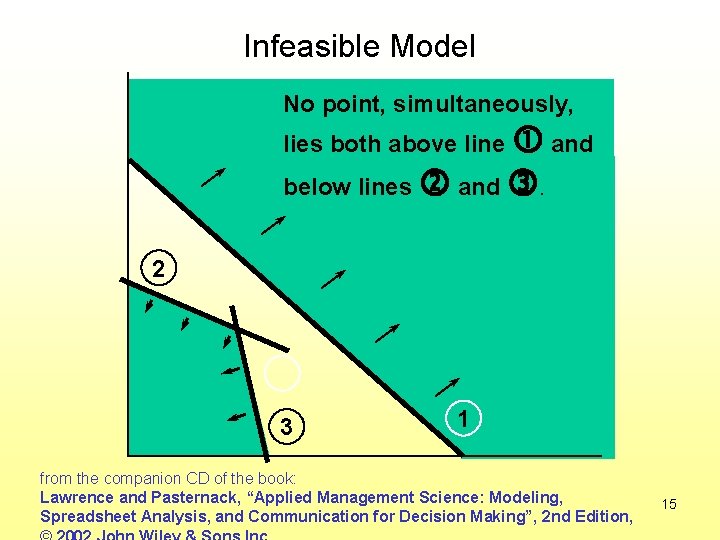
Special Situation in LP 2. Infeasibility: when no feasible solution exists (there is no feasible region) Example: x 1 < 10 x 1 > 15 14

Infeasible Model No point, simultaneously, lies both above line and below lines and . 2 3 1 from the companion CD of the book: Lawrence and Pasternack, “Applied Management Science: Modeling, Spreadsheet Analysis, and Communication for Decision Making”, 2 nd Edition, 15

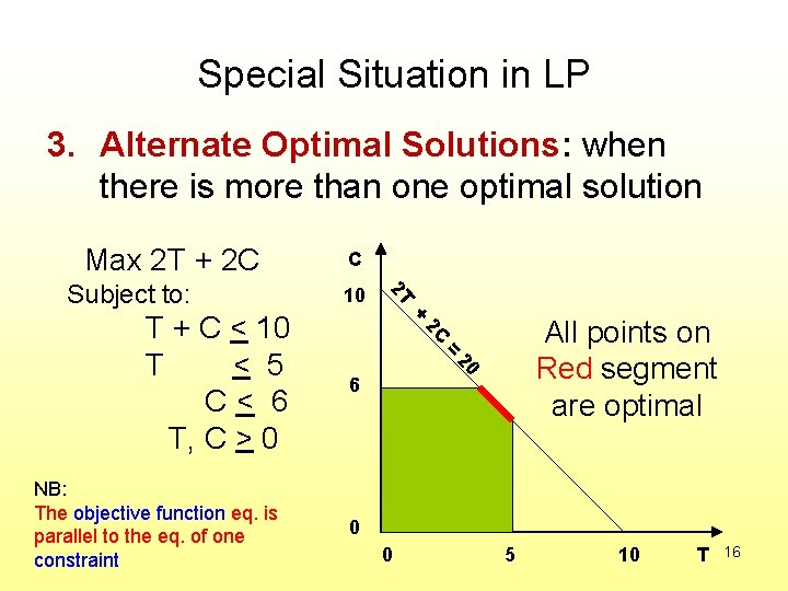
Special Situation in LP 3. Alternate Optimal Solutions: when there is more than one optimal solution Max 2 T + 2 C All points on Red segment are optimal 2 C = 20 NB: The objective function eq. is parallel to the eq. of one constraint + T + C < 10 T < 5 C< 6 T, C > 0 10 2 T Subject to: C 6 0 0 5 10 T 16

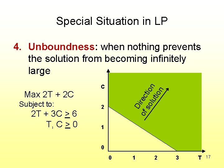
Special Situation in LP 4. Unboundness: when nothing prevents the solution from becoming infinitely large Subject to: 2 T + 3 C > 6 T, C > 0 Di of rec so tio lut n ion Max 2 T + 2 C C 2 1 0 0 1 2 3 T 17

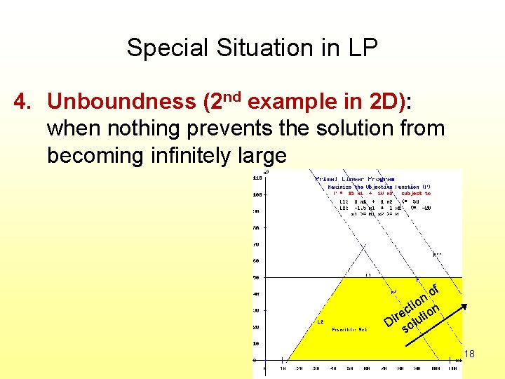
Special Situation in LP 4. Unboundness (2 nd example in 2 D): when nothing prevents the solution from becoming infinitely large f o on n i t c re lutio i D o s 18

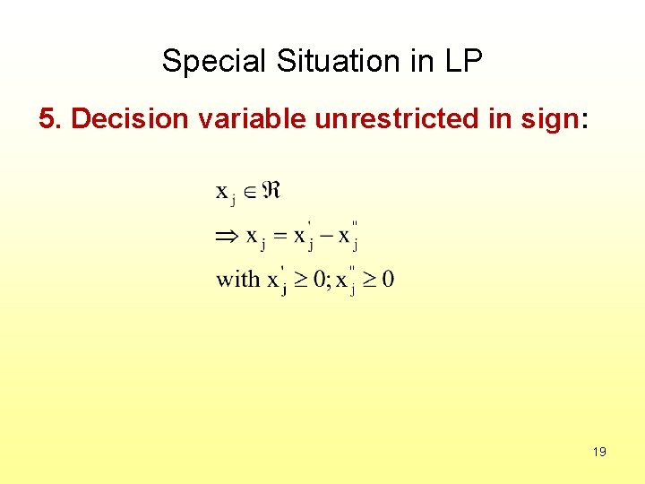
Special Situation in LP 5. Decision variable unrestricted in sign: 19

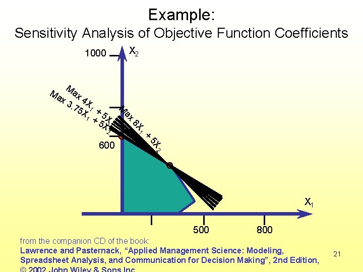
Sensitivity Analysis of the Optimal Solution • Is the optimal solution sensitive to changes in input parameters? • Possible reasons for asking this question: – Parameter values used were only best estimates. from the– companion CD of the book: Dynamic environment may cause changes. Lawrence and Pasternack, “Applied Management Science: Modeling, 20 Spreadsheet Analysis, and Communication for Decision Making”, 2 nd Edition, – “What-if” analysis may provide economical

Example: Sensitivity Analysis of Objective Function Coefficients X 2 1000 M Ma x 3 ax ax 8 X 1 2 M 4. 75 X 1 + X 5 X 1 + 5 X 2 + 5 X 600 2 X 1 500 800 from the companion CD of the book: Lawrence and Pasternack, “Applied Management Science: Modeling, Spreadsheet Analysis, and Communication for Decision Making”, 2 nd Edition, 21