Linear Programming Design of mathematical model 1 Formulating

- Slides: 33

Linear Programming Design of mathematical model 1

Formulating Linear Programming Model 1. decision variables These are the elements under the control of the decision-maker, and their values determine the solution of the model. 2. objective function – criterion function The decision maker will use it to evaluate alternative solutions to the problem. 3. Limitations These are the restrictions imposed upon the values of the decision variables. 4. Non negativity limits 2

Objective function • Two tipes: – Minimization • Costs, number of purchased good, kilometers – Maximization • Profit, benefit, utility 3

Limitations – Capacities or Capacity • Capacity of the storage • Capacity of machine • Capacity of sources – Requirements or Requirement • Requirements for the quantity of variables – Balance • Balance between the categories • Relationships in production – Definitional • Definition of 4

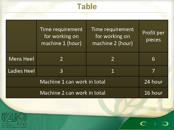
Example: Production • Enterprise produces two products for shoes– ladies heel and mens heel • Both of them has to be processed on two machines. The period of operation of machines is limited. • Requirements for working and working time machine is in the table. Establish a structure of production, during which the sale of products to achieve maximum profit. 5

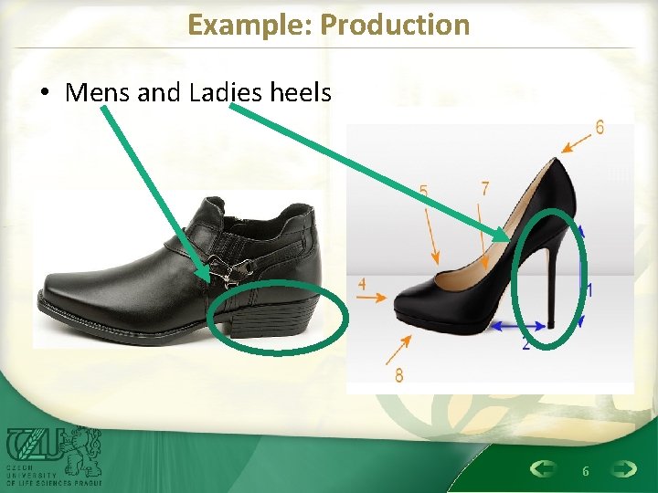
Example: Production • Mens and Ladies heels 6

Table Time requirement for working on machine 1 (hour) Time requirement for working on machine 2 (hour) Profit per pieces Mens Heel 2 2 6 Ladies Heel 3 1 7 Machine 1 can work in total 24 hour Machine 2 can work in total 16 hour 7

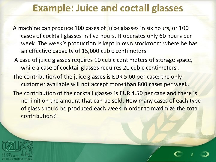
Example: Juice and coctail glasses A machine can produce 100 cases of juice glasses in six hours, or 100 cases of cocktail glasses in five hours. It operates only 60 hours per week. The week’s production is kept in own stockroom where he has an effective capacity of 15, 000 cubic centimeters. A case of juice glasses requires 10 cubic centimeters of storage space, while a case of cocktail glasses requires 20 cubic centimeters. The contribution of the juice glasses is EUR 5. 00 per case; the only customer available will not accept more than 800 cases per week. The contribution of the cocktail glasses is EUR 4. 50 per case and there is no limit on the amount that can be sold. How many cases of each type of glass should be produced each week in order to maximize the total contribution? 8

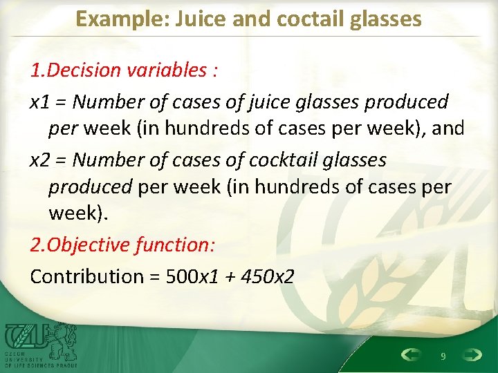
Example: Juice and coctail glasses 1. Decision variables : x 1 = Number of cases of juice glasses produced per week (in hundreds of cases per week), and x 2 = Number of cases of cocktail glasses produced per week (in hundreds of cases per week). 2. Objective function: Contribution = 500 x 1 + 450 x 2 9

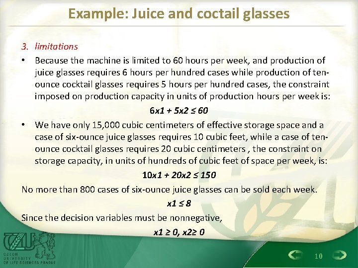
Example: Juice and coctail glasses 3. limitations • Because the machine is limited to 60 hours per week, and production of juice glasses requires 6 hours per hundred cases while production of tenounce cocktail glasses requires 5 hours per hundred cases, the constraint imposed on production capacity in units of production hours per week is: 6 x 1 + 5 x 2 ≤ 60 • We have only 15, 000 cubic centimeters of effective storage space and a case of six-ounce juice glasses requires 10 cubic feet, while a case of tenounce cocktail glasses requires 20 cubic centimeters , the constraint on storage capacity, in units of hundreds of cubic feet of space per week, is: 10 x 1 + 20 x 2 ≤ 150 No more than 800 cases of six-ounce juice glasses can be sold each week. x 1 ≤ 8 Since the decision variables must be nonnegative, x 1 ≥ 0, x 2≥ 0 10

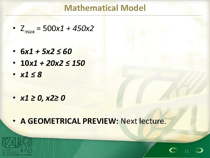
Mathematical Model • Zmax = 500 x 1 + 450 x 2 • 6 x 1 + 5 x 2 ≤ 60 • 10 x 1 + 20 x 2 ≤ 150 • x 1 ≤ 8 • x 1 ≥ 0, x 2≥ 0 • A GEOMETRICAL PREVIEW: Next lecture. 11

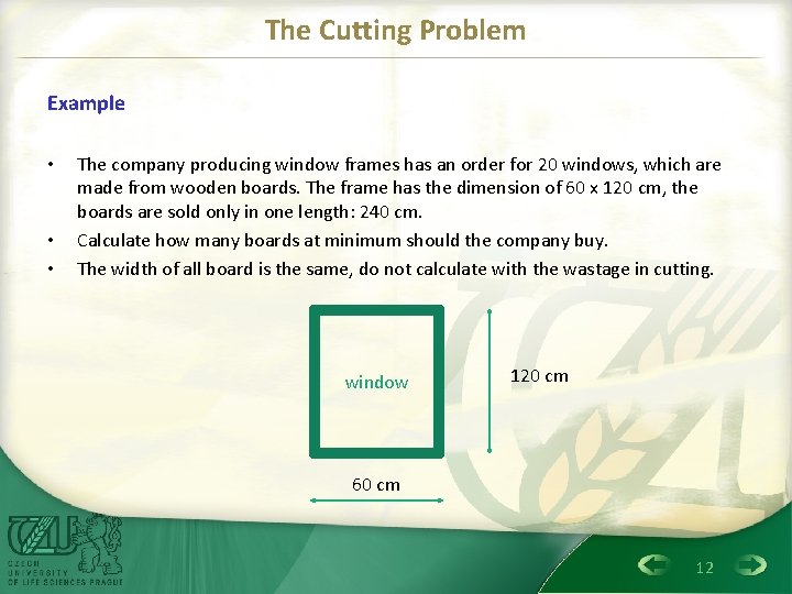
The Cutting Problem Example • • • The company producing window frames has an order for 20 windows, which are made from wooden boards. The frame has the dimension of 60 x 120 cm, the boards are sold only in one length: 240 cm. Calculate how many boards at minimum should the company buy. The width of all board is the same, do not calculate with the wastage in cutting. window 120 cm 60 cm 12

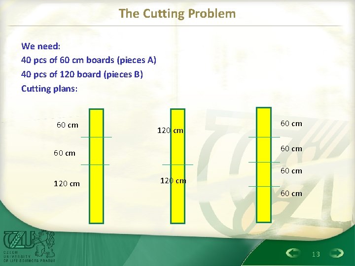
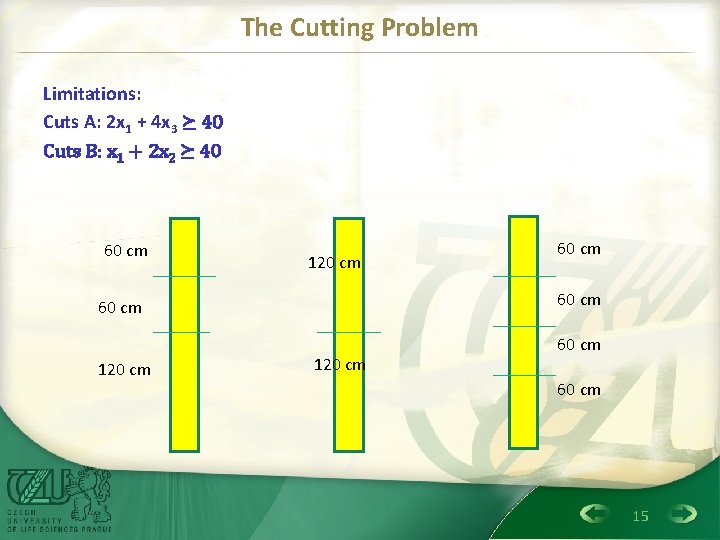
The Cutting Problem We need: 40 pcs of 60 cm boards (pieces A) 40 pcs of 120 board (pieces B) Cutting plans: 60 cm 120 cm 60 cm 13

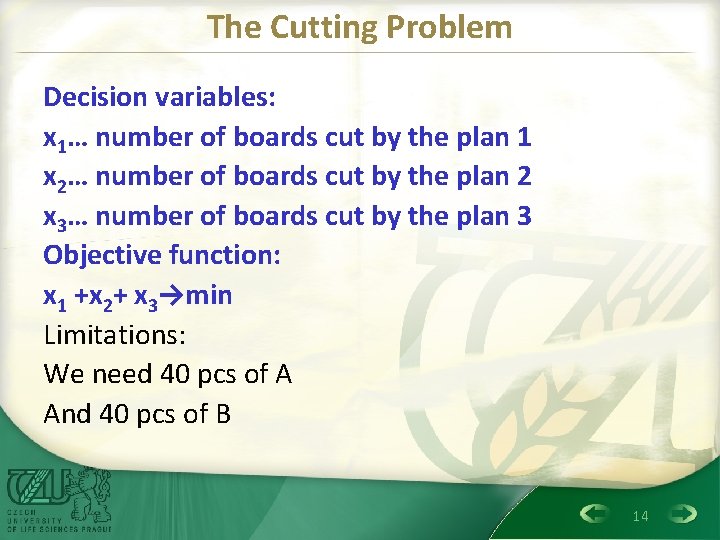
The Cutting Problem Decision variables: x 1… number of boards cut by the plan 1 x 2… number of boards cut by the plan 2 x 3… number of boards cut by the plan 3 Objective function: x 1 +x 2+ x 3→min Limitations: We need 40 pcs of A And 40 pcs of B 14

The Cutting Problem Limitations: Cuts A: 2 x 1 + 4 x 3 ⪰ 40 Cuts B: x 1 + 2 x 2 ⪰ 40 60 cm 120 cm 60 cm 15

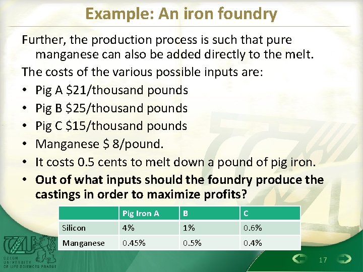
Example: An iron foundry • An iron foundry (slévárna) has a firm order to produce 1000 pounds of castings (odlitek) containing at least 0. 45 percent manganese and between 3. 25 percent and 5. 50 percent silicon. The castings sell for $0. 45 per pound. • The foundry has three types of pig iron available with the following properties: 16

Example: An iron foundry Further, the production process is such that pure manganese can also be added directly to the melt. The costs of the various possible inputs are: • Pig A $21/thousand pounds • Pig B $25/thousand pounds • Pig C $15/thousand pounds • Manganese $ 8/pound. • It costs 0. 5 cents to melt down a pound of pig iron. • Out of what inputs should the foundry produce the castings in order to maximize profits? Pig Iron A B C Silicon 4% 1% 0. 6% Manganese 0. 45% 0. 4% 17

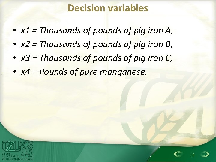
Decision variables • • x 1 = Thousands of pounds of pig iron A, x 2 = Thousands of pounds of pig iron B, x 3 = Thousands of pounds of pig iron C, x 4 = Pounds of pure manganese. 18

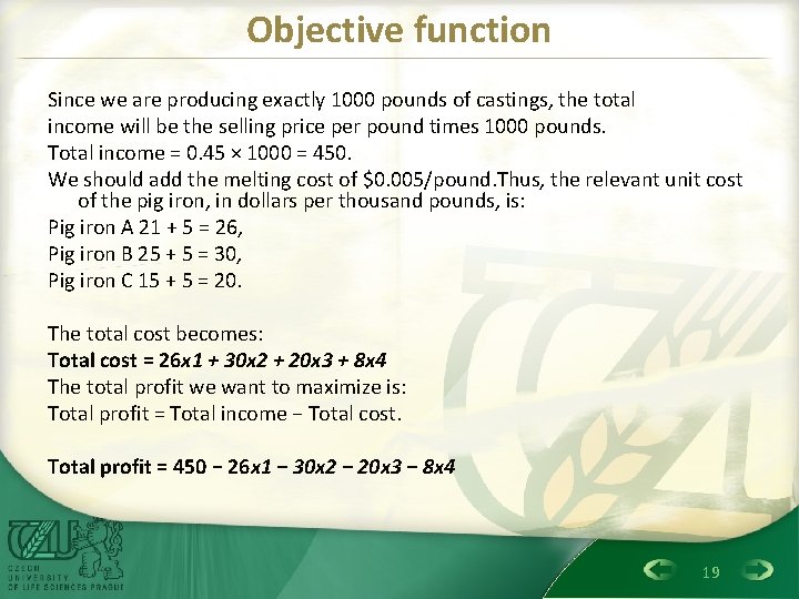
Objective function Since we are producing exactly 1000 pounds of castings, the total income will be the selling price per pound times 1000 pounds. Total income = 0. 45 × 1000 = 450. We should add the melting cost of $0. 005/pound. Thus, the relevant unit cost of the pig iron, in dollars per thousand pounds, is: Pig iron A 21 + 5 = 26, Pig iron B 25 + 5 = 30, Pig iron C 15 + 5 = 20. The total cost becomes: Total cost = 26 x 1 + 30 x 2 + 20 x 3 + 8 x 4 The total profit we want to maximize is: Total profit = Total income − Total cost. Total profit = 450 − 26 x 1 − 30 x 2 − 20 x 3 − 8 x 4 19

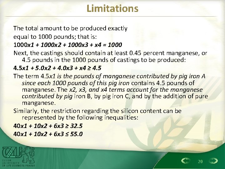
Limitations The total amount to be produced exactly equal to 1000 pounds; that is: 1000 x 1 + 1000 x 2 + 1000 x 3 + x 4 = 1000 Next, the castings should contain at least 0. 45 percent manganese, or 4. 5 pounds in the 1000 pounds of castings to be produced: 4. 5 x 1 + 5. 0 x 2 + 4. 0 x 3 + x 4 ≥ 4. 5 The term 4. 5 x 1 is the pounds of manganese contributed by pig iron A since each 1000 pounds of this pig iron contains 4. 5 pounds of manganese. The x 2, x 3, and x 4 terms account for the manganese contributed by pig iron B, by pig iron C, and by the addition of pure manganese. Similarly, the restriction regarding the silicon content can be represented by the following inequalities: 40 x 1 + 10 x 2 + 6 x 3 ≥ 32. 5 40 x 1 + 10 x 2 + 6 x 3 ≤ 55. 0 20

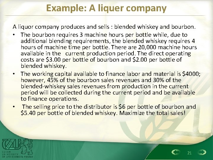
Example: A liquer company A liquor company produces and sells : blended whiskey and bourbon. • The bourbon requires 3 machine hours per bottle while, due to additional blending requirements, the blended whiskey requires 4 hours of machine time per bottle. There are 20, 000 machine hours available in the current production period. The direct operating costs are $3. 00 per bottle of bourbon and $2. 00 per bottle of blended whiskey. • The working capital available to finance labor and material is $4000; however, 45% of the bourbon sales revenues and 30% of the blended-whiskey sales revenues from production in the current period will be collected during the current period and be available to finance operations. • The selling price to the distributor is $6 per bottle of bourbon and $5. 40 per bottle of blended whiskey. Maximize the total sales! 21

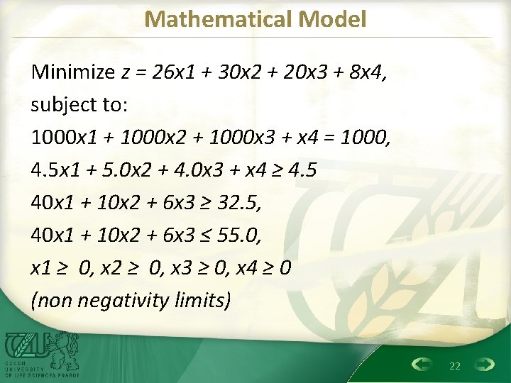
Mathematical Model Minimize z = 26 x 1 + 30 x 2 + 20 x 3 + 8 x 4, subject to: 1000 x 1 + 1000 x 2 + 1000 x 3 + x 4 = 1000, 4. 5 x 1 + 5. 0 x 2 + 4. 0 x 3 + x 4 ≥ 4. 5 40 x 1 + 10 x 2 + 6 x 3 ≥ 32. 5, 40 x 1 + 10 x 2 + 6 x 3 ≤ 55. 0, x 1 ≥ 0, x 2 ≥ 0, x 3 ≥ 0, x 4 ≥ 0 (non negativity limits) 22

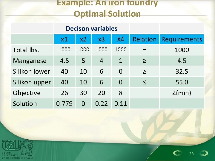
Example: An iron foundry Optimal Solution Decison variables x 1 x 2 x 3 X 4 Total lbs. Manganese Relation Requirements 1000 = 1000 4. 5 5 4 1 ≥ 4. 5 Silikon lower 40 Silikon upper 40 Objective 26 Solution 0. 779 10 10 30 0 6 0 20 8 0. 22 0. 11 ≥ ≤ 32. 5 55. 0 Z(min) 23

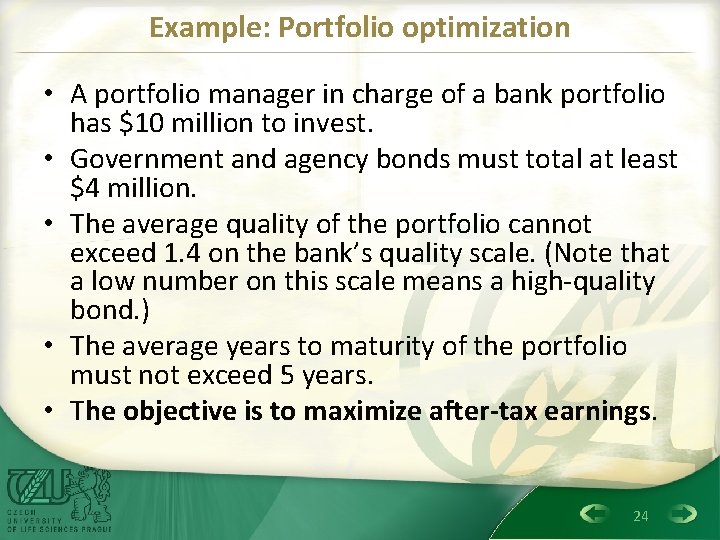
Example: Portfolio optimization • A portfolio manager in charge of a bank portfolio has $10 million to invest. • Government and agency bonds must total at least $4 million. • The average quality of the portfolio cannot exceed 1. 4 on the bank’s quality scale. (Note that a low number on this scale means a high-quality bond. ) • The average years to maturity of the portfolio must not exceed 5 years. • The objective is to maximize after-tax earnings. 24

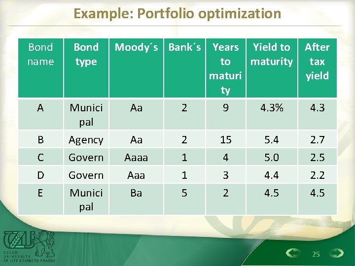
Example: Portfolio optimization Bond name Bond type Moody´s Bank´s Years Yield to After to maturity tax maturi yield ty Aa 2 9 4. 3% 4. 3 A Munici pal B C Agency Govern Aa Aaaa 2 1 15 4 5. 0 2. 7 2. 5 D E Govern Munici pal Aaa Ba 1 5 3 2 4. 4 4. 5 2. 2 4. 5 25

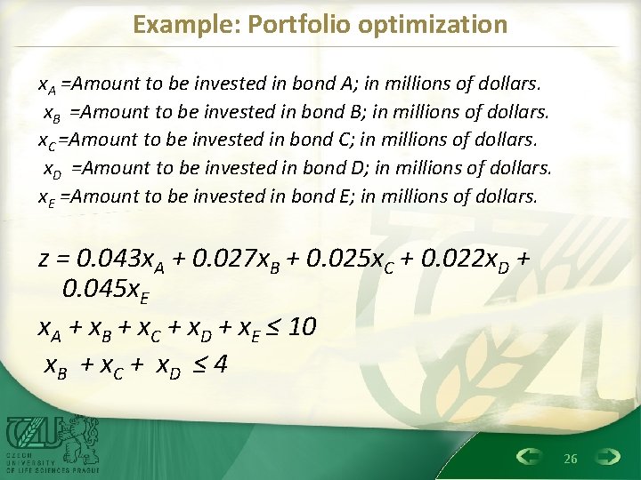
Example: Portfolio optimization x. A =Amount to be invested in bond A; in millions of dollars. x. B =Amount to be invested in bond B; in millions of dollars. x. C =Amount to be invested in bond C; in millions of dollars. x. D =Amount to be invested in bond D; in millions of dollars. x. E =Amount to be invested in bond E; in millions of dollars. z = 0. 043 x. A + 0. 027 x. B + 0. 025 x. C + 0. 022 x. D + 0. 045 x. E x. A + x. B + x. C + x. D + x. E ≤ 10 x B + x. C + x D ≤ 4 26

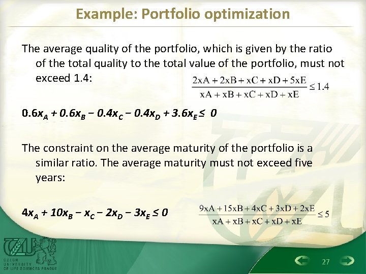
Example: Portfolio optimization The average quality of the portfolio, which is given by the ratio of the total quality to the total value of the portfolio, must not exceed 1. 4: 0. 6 x. A + 0. 6 x. B − 0. 4 x. C − 0. 4 x. D + 3. 6 x. E ≤ 0 The constraint on the average maturity of the portfolio is a similar ratio. The average maturity must not exceed five years: 4 x. A + 10 x. B − x. C − 2 x. D − 3 x. E ≤ 0 27

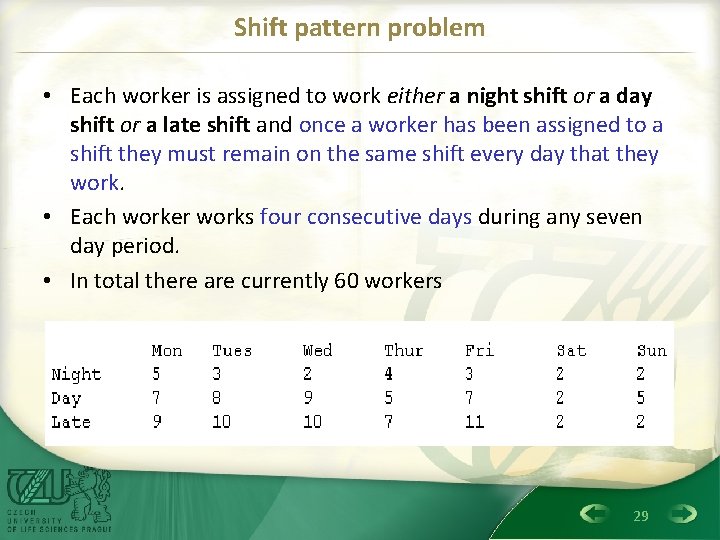
LP: Basic Groups of Applications Shift pattern problem: The production manager of a chemical plant is attempting to devise a shift pattern for his workforce. Each day of every working week is divided into three eight-hour shift periods (00: 01 -08: 00, 08: 01 -16: 00, 16: 01 -24: 00) denoted by night, day and late respectively. The plant must be manned at all times and the minimum number of workers required for each of these shifts over any working week is on the next slide: 28

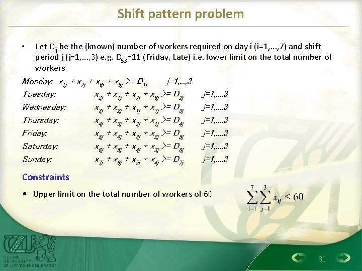
Shift pattern problem • Each worker is assigned to work either a night shift or a day shift or a late shift and once a worker has been assigned to a shift they must remain on the same shift every day that they work. • Each worker works four consecutive days during any seven day period. • In total there are currently 60 workers 29

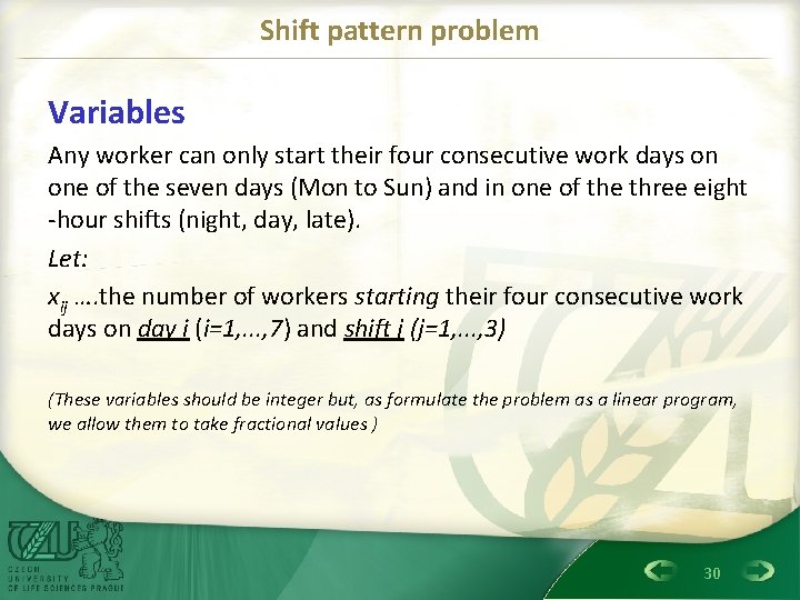
Shift pattern problem Variables Any worker can only start their four consecutive work days on one of the seven days (Mon to Sun) and in one of the three eight -hour shifts (night, day, late). Let: xij …. the number of workers starting their four consecutive work days on day i (i=1, . . . , 7) and shift j (j=1, . . . , 3) (These variables should be integer but, as formulate the problem as a linear program, we allow them to take fractional values ) 30

Shift pattern problem • Let Dij be the (known) number of workers required on day i (i=1, . . . , 7) and shift period j (j=1, . . . , 3) e. g. D 53=11 (Friday, Late) i. e. lower limit on the total number of workers Monday: x 1 j + x 7 j + x 6 j + x 5 j >= D 1 j j=1, . . . , 3 Tuesday: x 2 j + x 1 j + x 7 j + x 6 j >= D 2 j Wednesday: x 3 j + x 2 j + x 1 j + x 7 j >= D 3 j Thursday: x 4 j + x 3 j + x 2 j + x 1 j >= D 4 j Friday: x 5 j + x 4 j + x 3 j + x 2 j >= D 5 j Saturday: x 6 j + x 5 j + x 4 j + x 3 j >= D 6 j Sunday: x 7 j + x 6 j + x 5 j + x 4 j >= D 7 j j=1, . . . , 3 Constraints • Upper limit on the total number of workers of 60 31

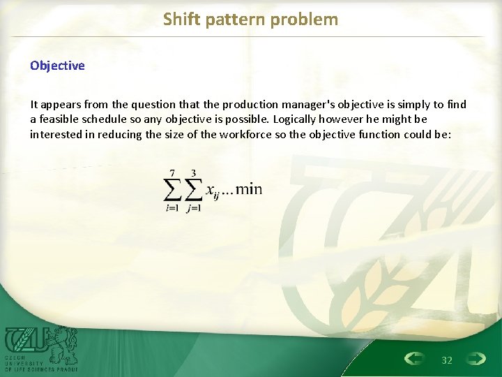
Shift pattern problem Objective It appears from the question that the production manager's objective is simply to find a feasible schedule so any objective is possible. Logically however he might be interested in reducing the size of the workforce so the objective function could be: 32

Summary • Linear programming mathematical model • Decision variables definition • 3 parts of model: – Objective (target) function – Limits – Nonnegativity limites • Percentage • Bilance conditions 33