Linear Programming Contents Introduction History Applications Linear programming

Linear Programming

Contents • • • Introduction History Applications Linear programming model Example of Linear Programming Problems Graphical Solution to Linear Programming Problem • Sensitivity analysis 2

Introduction • Linear Programming is a mathematical modeling technique used to determine a level of operational activity in order to achieve an objective. • Mathematical programming is used to find the best or optimal solution to a problem that requires a decision or set of decisions about how best to use a set of limited resources to achieve a state goal of objectives. 3

• Steps involved in mathematical programming – Conversion of stated problem into a mathematical model that abstracts all the essential elements of the problem. – Exploration of different solutions of the problem. – Find out the most suitable or optimum solution. • Linear programming requires that all the mathematical functions in the model be linear functions. 4

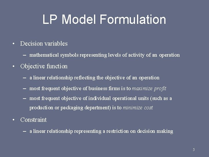
LP Model Formulation • Decision variables – mathematical symbols representing levels of activity of an operation • Objective function – a linear relationship reflecting the objective of an operation – most frequent objective of business firms is to maximize profit – most frequent objective of individual operational units (such as a production or packaging department) is to minimize cost • Constraint – a linear relationship representing a restriction on decision making 5

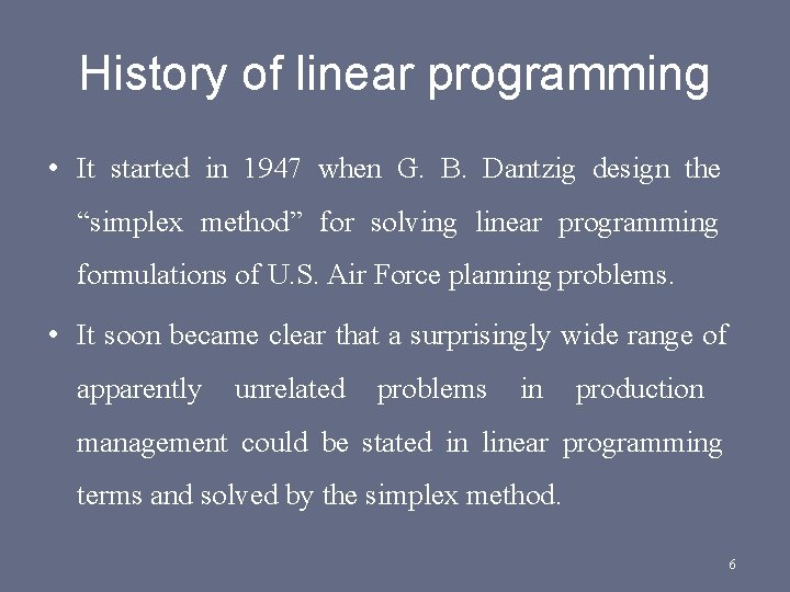
History of linear programming • It started in 1947 when G. B. Dantzig design the “simplex method” for solving linear programming formulations of U. S. Air Force planning problems. • It soon became clear that a surprisingly wide range of apparently unrelated problems in production management could be stated in linear programming terms and solved by the simplex method. 6

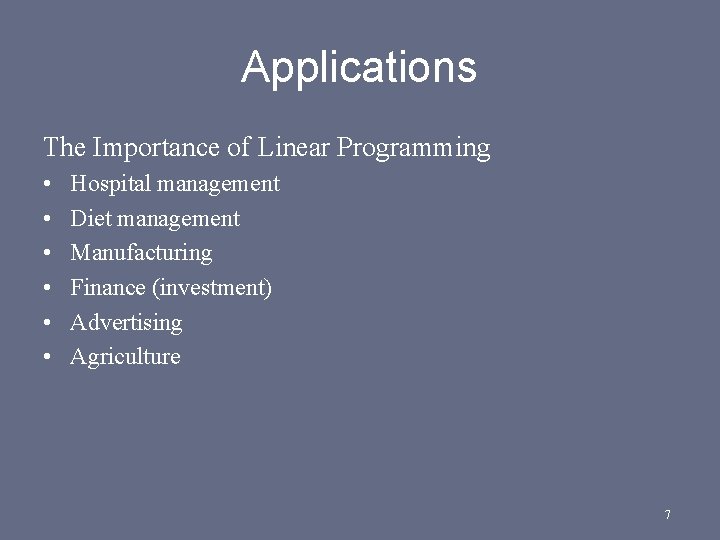
Applications The Importance of Linear Programming • • • Hospital management Diet management Manufacturing Finance (investment) Advertising Agriculture 7

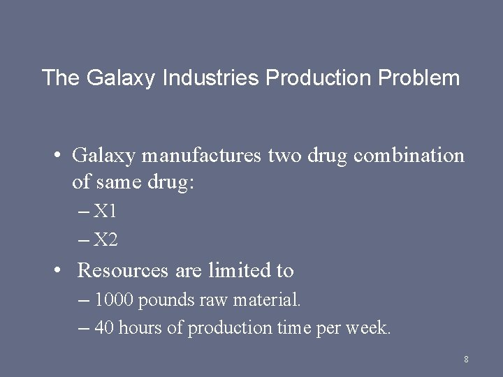
The Galaxy Industries Production Problem • Galaxy manufactures two drug combination of same drug: – X 1 – X 2 • Resources are limited to – 1000 pounds raw material. – 40 hours of production time per week. 8

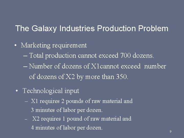
The Galaxy Industries Production Problem • Marketing requirement – Total production cannot exceed 700 dozens. – Number of dozens of X 1 cannot exceed number of dozens of X 2 by more than 350. • Technological input – X 1 requires 2 pounds of raw material and 3 minutes of labor per dozen. – X 2 requires 1 pound of raw material and 4 minutes of labor per dozen. 9

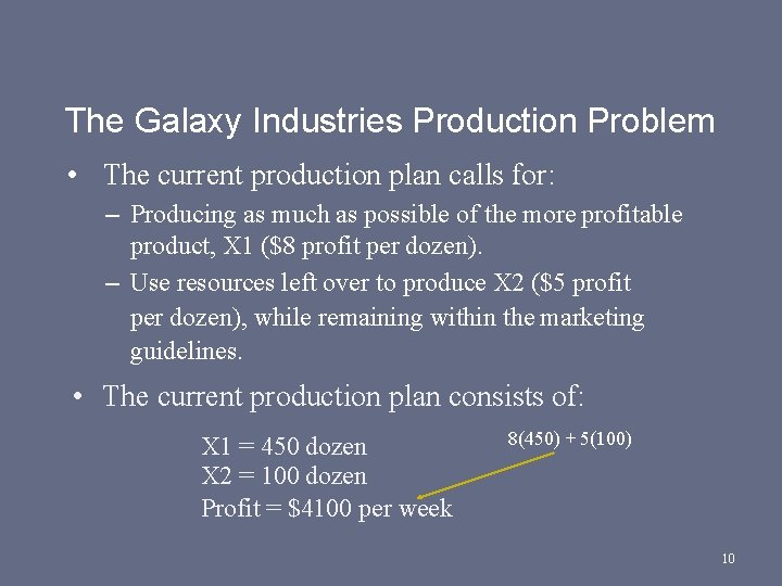
The Galaxy Industries Production Problem • The current production plan calls for: – Producing as much as possible of the more profitable product, X 1 ($8 profit per dozen). – Use resources left over to produce X 2 ($5 profit per dozen), while remaining within the marketing guidelines. • The current production plan consists of: X 1 = 450 dozen X 2 = 100 dozen Profit = $4100 per week 8(450) + 5(100) 10

Management is seeking a production schedule that will increase the company’s profit. 11

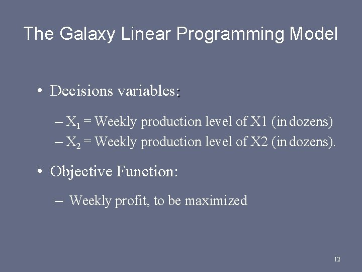
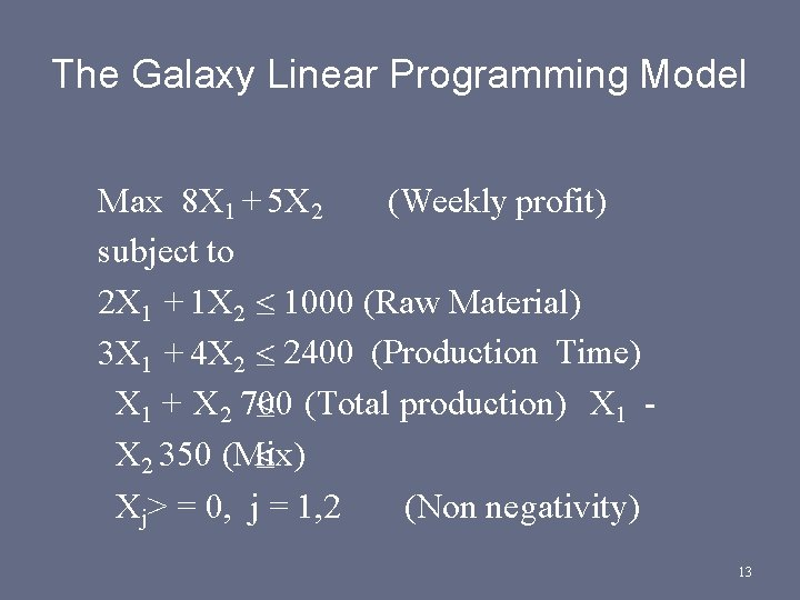
The Galaxy Linear Programming Model • Decisions variables: – X 1 = Weekly production level of X 1 (in dozens) – X 2 = Weekly production level of X 2 (in dozens). • Objective Function: – Weekly profit, to be maximized 12

The Galaxy Linear Programming Model Max 8 X 1 + 5 X 2 (Weekly profit) subject to 2 X 1 + 1 X 2 1000 (Raw Material) 3 X 1 + 4 X 2 2400 (Production Time) X 1 + X 2 700 (Total production) X 1 X 2 350 (Mix) Xj> = 0, j = 1, 2 (Non negativity) 13

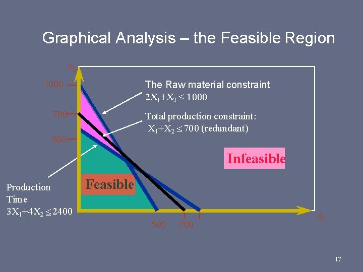
The Graphical Analysis of Linear Programming The set of all points that satisfy all the constraints of the model is called a FEASIBLE REGION 14

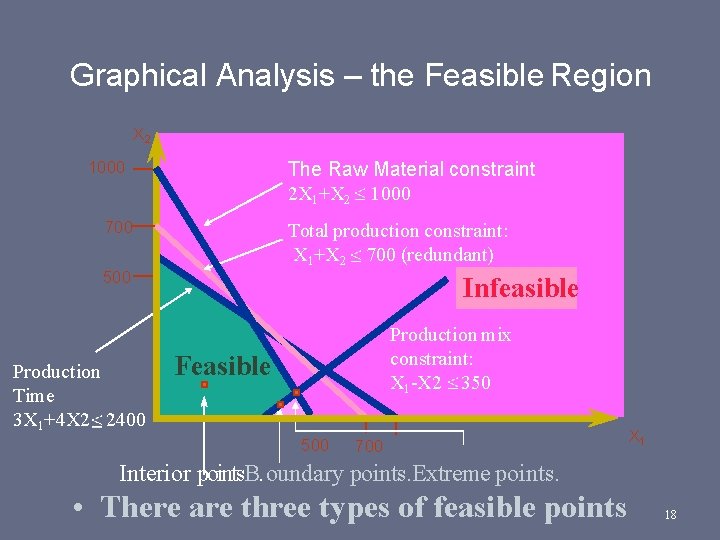
Using a graphical presentation we can represent all the constraints, the objective function, and the three types of feasible points. 15

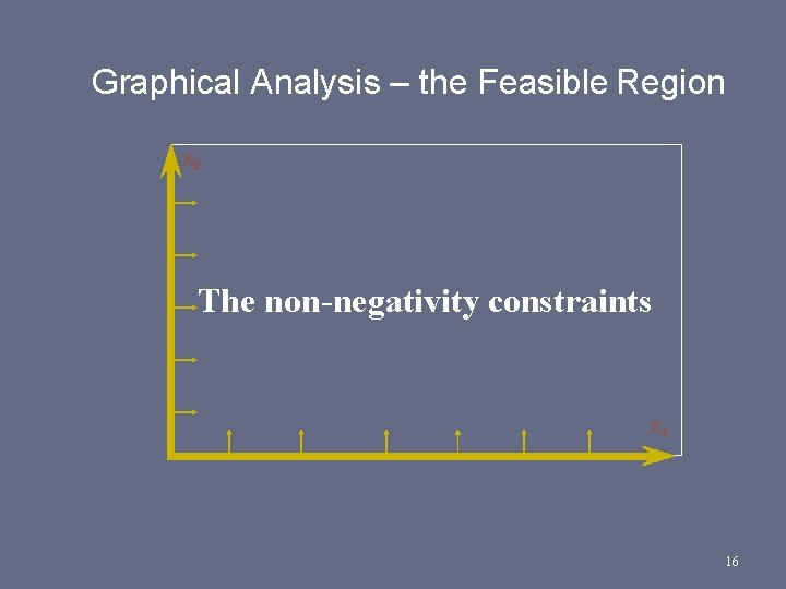
Graphical Analysis – the Feasible Region X 2 The non-negativity constraints X 1 16

Graphical Analysis – the Feasible Region X 2 The Raw material constraint 2 X 1+X 2 1000 700 Total production constraint: X 1+X 2 700 (redundant) 500 Infeasible Production Time 3 X 1+4 X 2 2400 Feasible 500 700 X 1 17

Graphical Analysis – the Feasible Region X 2 The Raw Material constraint 2 X 1+X 2 1000 700 Total production constraint: X 1+X 2 700 (redundant) 500 Production Time 3 X 1+4 X 2 2400 Infeasible Production mix constraint: X 1 -X 2 350 Feasible 500 700 X 1 Interior points. B. oundary points. Extreme points. • There are three types of feasible points 18

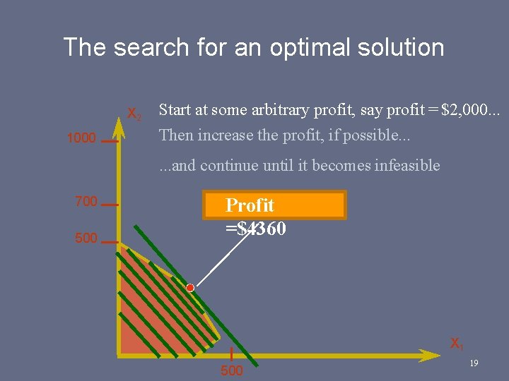
The search for an optimal solution X 2 1000 Start at some arbitrary profit, say profit = $2, 000. . . Then increase the profit, if possible. . . and continue until it becomes infeasible 700 500 Profit =$4360 X 1 500 19

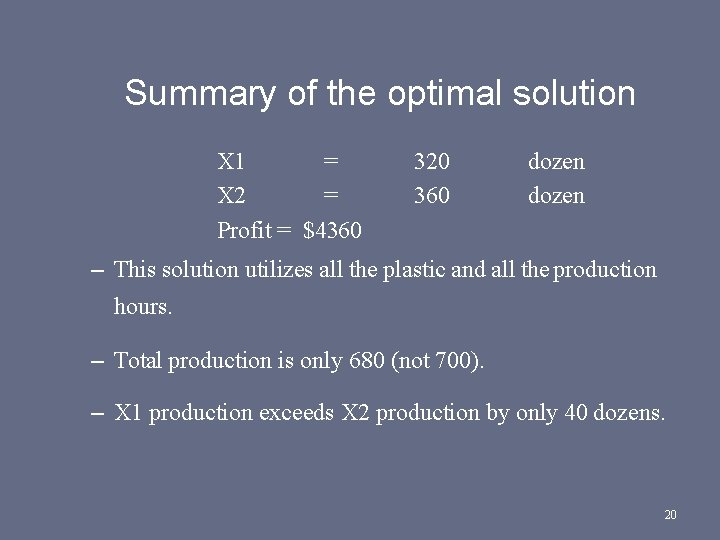
Summary of the optimal solution X 1 = X 2 = Profit = $4360 320 360 dozen – This solution utilizes all the plastic and all the production hours. – Total production is only 680 (not 700). – X 1 production exceeds X 2 production by only 40 dozens. 20

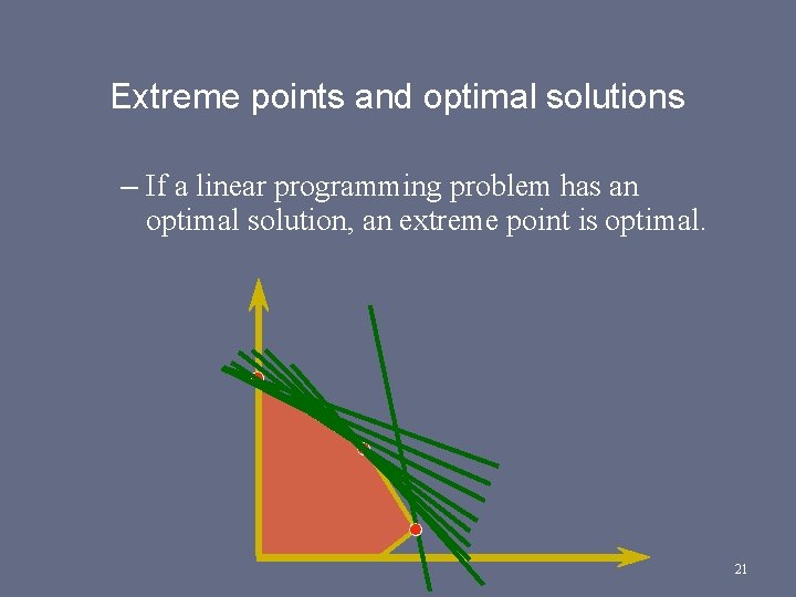
Extreme points and optimal solutions – If a linear programming problem has an optimal solution, an extreme point is optimal. 21

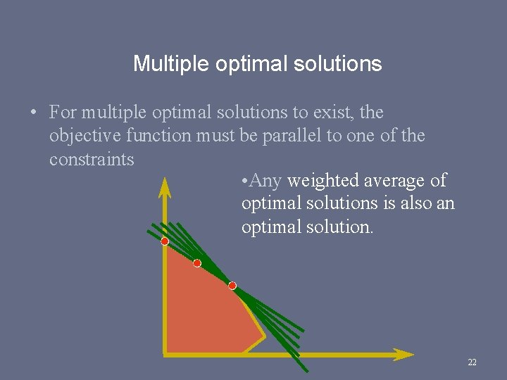
Multiple optimal solutions • For multiple optimal solutions to exist, the objective function must be parallel to one of the constraints • Any weighted average of optimal solutions is also an optimal solution. 22

Sensitivity Analysis of the Optimal Solution • Is the optimal solution sensitive to changes in input parameters? • Possible reasons for asking this question: – Parameter values used were only best estimates. – Dynamic environment may cause changes. – “What-if” analysis may provide economical and operational information. 23

Sensitivity Analysis of Objective Function Coefficients. • Range of Optimality – The optimal solution will remain unchanged as long as • An objective function coefficient lies within its range of optimality • There are no changes in any other input parameters. – The value of the objective function will change if the coefficient multiplies a variable whose value is nonzero. 24

25

REFERENCES • • • www. math. ucla. edu/~tom/LP. pdf www. sce. carleton. ca/faculty/chinneck/po/Chapter 2. www. markschulze. net/Linear. Programming. pdf web. ntpu. edu. tw/~juang/ms/Ch 02. cmp. felk. cvut. cz/~hlavac/Public/. . . /Linear%20 Progra mming-1. ppt • www. slideshare. net/nagendraamatya/linearprogramming 26

27