LINEAR PROG A Model Example Let us consider

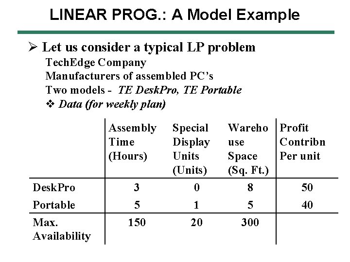
LINEAR PROG. : A Model Example Ø Let us consider a typical LP problem Tech. Edge Company Manufacturers of assembled PC’s Two models - TE Desk. Pro, TE Portable v Data (for weekly plan) Assembly Time (Hours) Special Display Units (Units) Wareho Profit use Contribn Space Per unit (Sq. Ft. ) Desk. Pro 3 0 8 50 Portable 5 1 5 40 150 20 300 Max. Availability

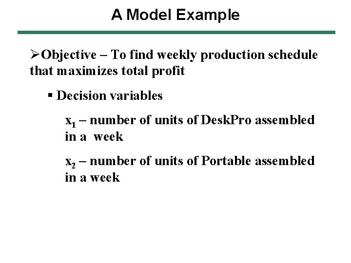
A Model Example ØObjective – To find weekly production schedule that maximizes total profit § Decision variables x 1 – number of units of Desk. Pro assembled in a week x 2 – number of units of Portable assembled in a week

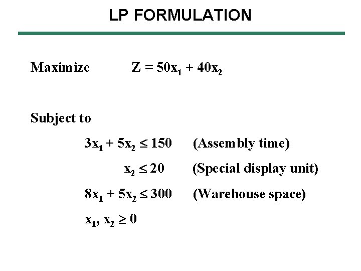
LP FORMULATION Maximize Z = 50 x 1 + 40 x 2 Subject to 3 x 1 + 5 x 2 150 x 2 20 8 x 1 + 5 x 2 300 x 1, x 2 0 (Assembly time) (Special display unit) (Warehouse space)

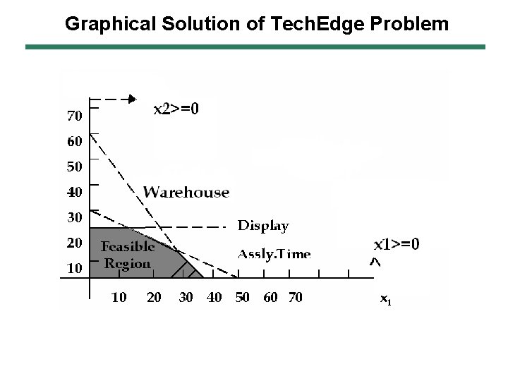
Graphical Solution of Tech. Edge Problem

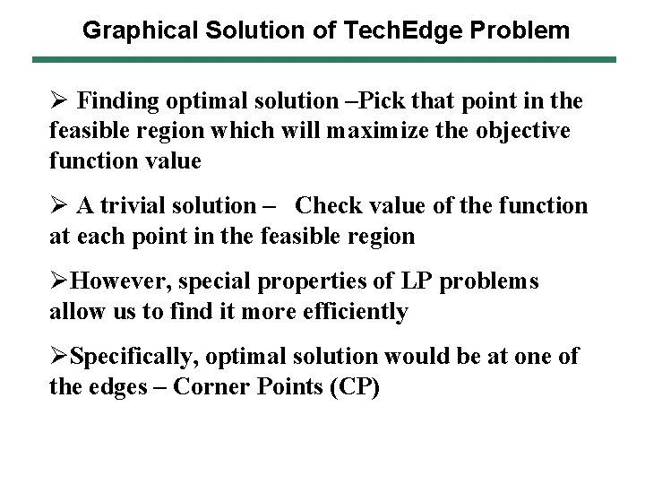
Graphical Solution of Tech. Edge Problem Ø Finding optimal solution –Pick that point in the feasible region which will maximize the objective function value Ø A trivial solution – Check value of the function at each point in the feasible region ØHowever, special properties of LP problems allow us to find it more efficiently ØSpecifically, optimal solution would be at one of the edges – Corner Points (CP)

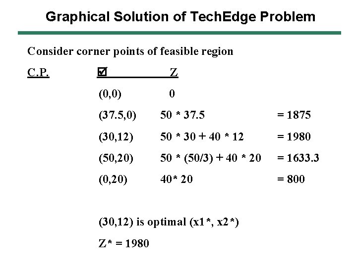
Graphical Solution of Tech. Edge Problem Consider corner points of feasible region C. P. Z (0, 0) 0 (37. 5, 0) 50 * 37. 5 = 1875 (30, 12) 50 * 30 + 40 * 12 = 1980 (50, 20) 50 * (50/3) + 40 * 20 = 1633. 3 (0, 20) 40* 20 = 800 (30, 12) is optimal (x 1*, x 2*) Z* = 1980

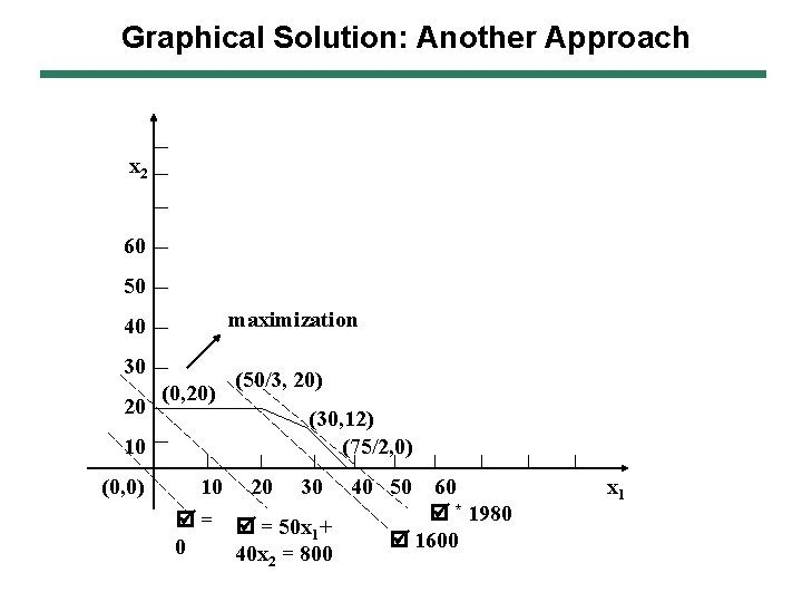
Graphical Solution: Another Approach x 2 60 50 maximization 40 30 20 (0, 20) (50/3, 20) (30, 12) (75/2, 0) 10 (0, 0) 10 20 30 = = 50 x + 1 0 40 x 2 = 800 40 50 60 * 1980 1600 x 1

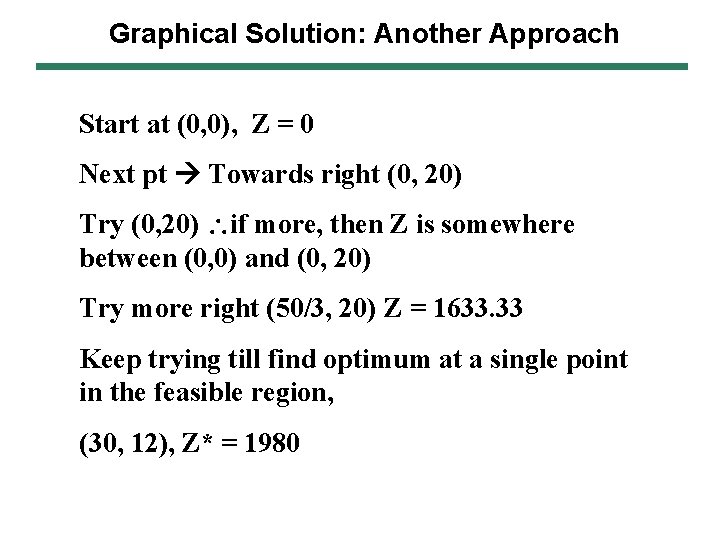
Graphical Solution: Another Approach Start at (0, 0), Z = 0 Next pt Towards right (0, 20) Try (0, 20) if more, then Z is somewhere between (0, 0) and (0, 20) Try more right (50/3, 20) Z = 1633. 33 Keep trying till find optimum at a single point in the feasible region, (30, 12), Z* = 1980

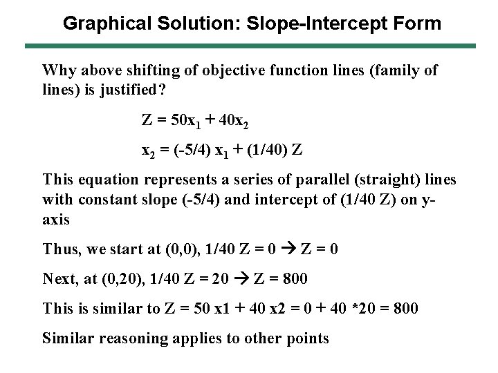
Graphical Solution: Slope-Intercept Form Why above shifting of objective function lines (family of lines) is justified? Z = 50 x 1 + 40 x 2 = (-5/4) x 1 + (1/40) Z This equation represents a series of parallel (straight) lines with constant slope (-5/4) and intercept of (1/40 Z) on yaxis Thus, we start at (0, 0), 1/40 Z = 0 Next, at (0, 20), 1/40 Z = 20 Z = 800 This is similar to Z = 50 x 1 + 40 x 2 = 0 + 40 *20 = 800 Similar reasoning applies to other points

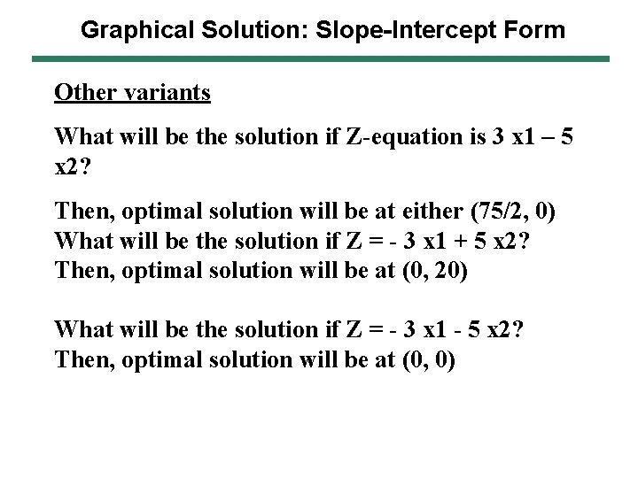
Graphical Solution: Slope-Intercept Form Other variants What will be the solution if Z-equation is 3 x 1 – 5 x 2? Then, optimal solution will be at either (75/2, 0) What will be the solution if Z = - 3 x 1 + 5 x 2? Then, optimal solution will be at (0, 20) What will be the solution if Z = - 3 x 1 - 5 x 2? Then, optimal solution will be at (0, 0)

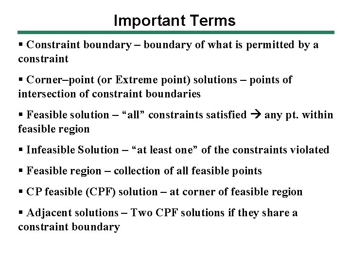
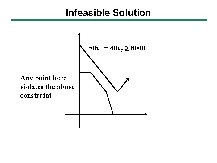
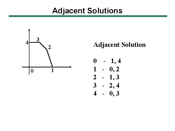
Important Terms § Constraint boundary – boundary of what is permitted by a constraint § Corner–point (or Extreme point) solutions – points of intersection of constraint boundaries § Feasible solution – “all” constraints satisfied any pt. within feasible region § Infeasible Solution – “at least one” of the constraints violated § Feasible region – collection of all feasible points § CP feasible (CPF) solution – at corner of feasible region § Adjacent solutions – Two CPF solutions if they share a constraint boundary

Infeasible Solution 50 x 1 + 40 x 2 8000 Any point here violates the above constraint

Adjacent Solutions 3 4 Adjacent Solution 2 0 1 2 3 4 - 1, 4 0, 2 1, 3 2, 4 0, 3

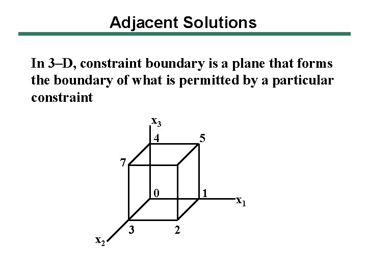
Adjacent Solutions In 3–D, constraint boundary is a plane that forms the boundary of what is permitted by a particular constraint x 3 4 5 0 1 7 x 2 3 2 x 1

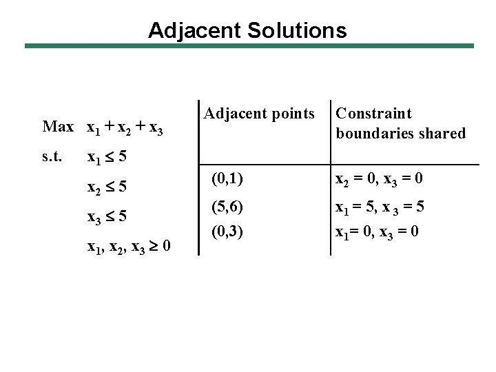
Adjacent Solutions Max x 1 + x 2 + x 3 s. t. Adjacent points Constraint boundaries shared x 1 5 x 2 5 x 3 5 x 1, x 2, x 3 0 (0, 1) x 2 = 0, x 3 = 0 (5, 6) x 1 = 5, x 3 = 5 (0, 3) x 1= 0, x 3 = 0

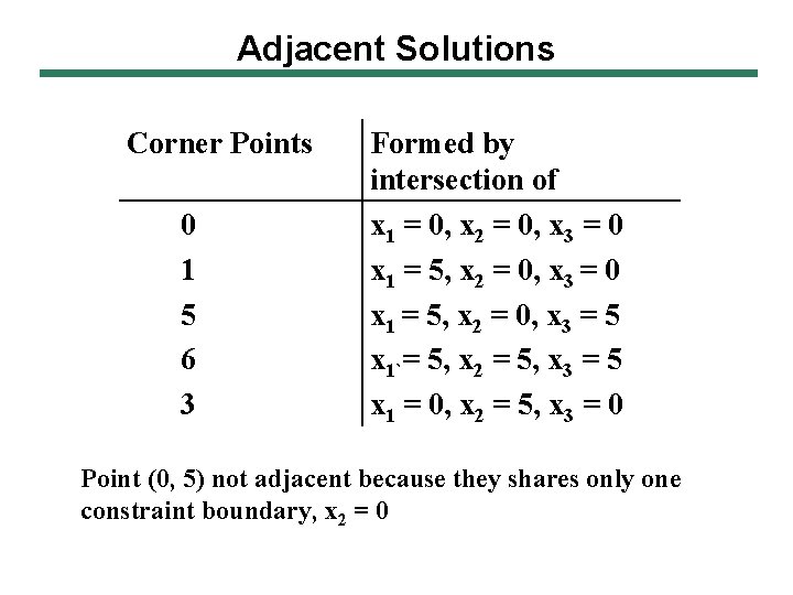
Adjacent Solutions Corner Points 0 1 5 6 3 Formed by intersection of x 1 = 0, x 2 = 0, x 3 = 0 x 1 = 5, x 2 = 0, x 3 = 5 x 1`= 5, x 2 = 5, x 3 = 5 x 1 = 0, x 2 = 5, x 3 = 0 Point (0, 5) not adjacent because they shares only one constraint boundary, x 2 = 0

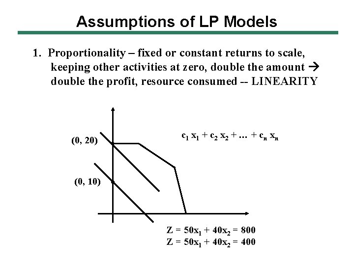
Assumptions of LP Models 1. Proportionality – fixed or constant returns to scale, keeping other activities at zero, double the amount double the profit, resource consumed -- LINEARITY (0, 20) c 1 x 1 + c 2 x 2 + … + cn xn (0, 10) Z = 50 x 1 + 40 x 2 = 800 Z = 50 x 1 + 40 x 2 = 400

Assumptions of LP Models 2. Additivity – Total profit / consumption of resources = Sum of individual profit / consumptions no interactive (multiplicative) or non-linear terms allowed 3. Divisibility – Continuous (or non-integer) values possible 4. Deterministic – all parameters of the model are known

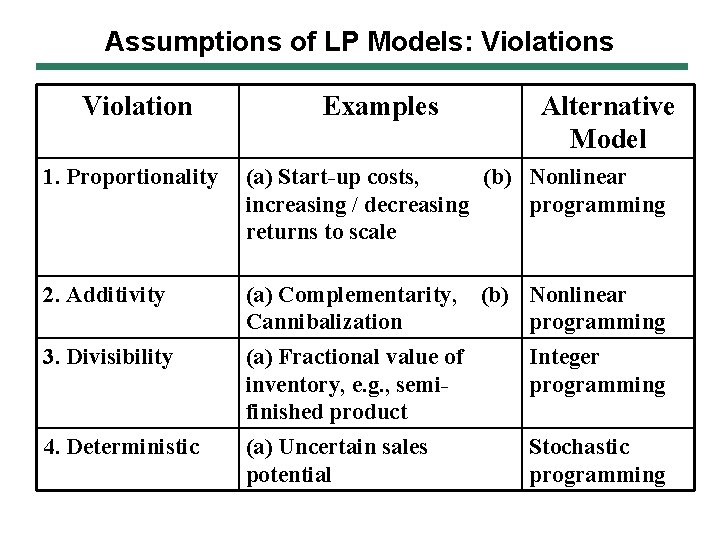
Assumptions of LP Models: Violations Violation Examples Alternative Model 1. Proportionality (a) Start-up costs, (b) Nonlinear increasing / decreasing programming returns to scale 2. Additivity (a) Complementarity, Cannibalization (b) Nonlinear programming 3. Divisibility (a) Fractional value of inventory, e. g. , semifinished product Integer programming 4. Deterministic (a) Uncertain sales potential Stochastic programming

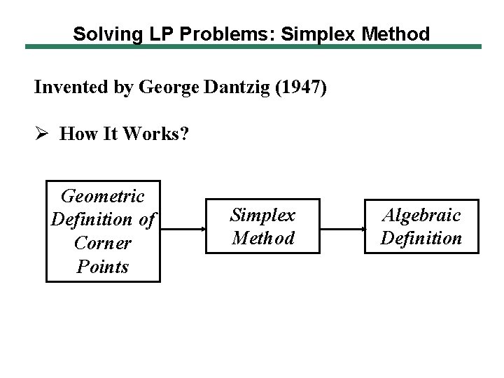
Solving LP Problems: Simplex Method Invented by George Dantzig (1947) Ø How It Works? Geometric Definition of Corner Points Simplex Method Algebraic Definition

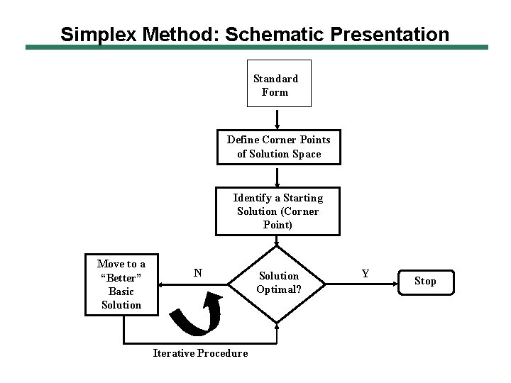
Simplex Method: Schematic Presentation Standard Form Define Corner Points of Solution Space Identify a Starting Solution (Corner Point) Move to a “Better” Basic Solution N Iterative Procedure Solution Optimal? Y Stop

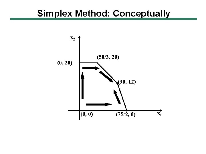
Simplex Method: Conceptually x 2 (50/3, 20) (0, 20) (30, 12) (0, 0) (75/2, 0) x 1

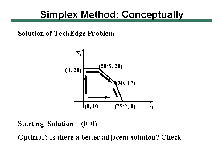
Simplex Method: Conceptually Solution of Tech. Edge Problem x 2 (50/3, 20) (0, 20) (30, 12) (0, 0) (75/2, 0) x 1 Starting Solution – (0, 0) Optimal? Is there a better adjacent solution? Check

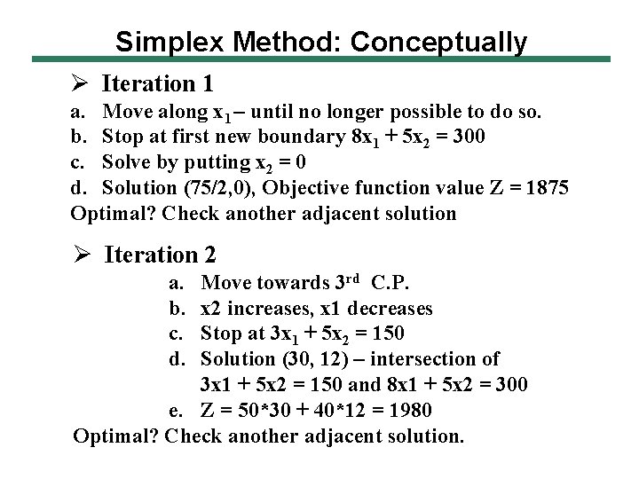
Simplex Method: Conceptually Ø Iteration 1 a. Move along x 1 – until no longer possible to do so. b. Stop at first new boundary 8 x 1 + 5 x 2 = 300 c. Solve by putting x 2 = 0 d. Solution (75/2, 0), Objective function value Z = 1875 Optimal? Check another adjacent solution Ø Iteration 2 a. b. c. d. Move towards 3 rd C. P. x 2 increases, x 1 decreases Stop at 3 x 1 + 5 x 2 = 150 Solution (30, 12) – intersection of 3 x 1 + 5 x 2 = 150 and 8 x 1 + 5 x 2 = 300 e. Z = 50*30 + 40*12 = 1980 Optimal? Check another adjacent solution.

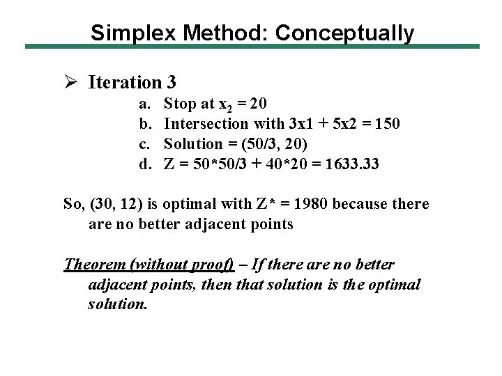
Simplex Method: Conceptually Ø Iteration 3 a. b. c. d. Stop at x 2 = 20 Intersection with 3 x 1 + 5 x 2 = 150 Solution = (50/3, 20) Z = 50*50/3 + 40*20 = 1633. 33 So, (30, 12) is optimal with Z* = 1980 because there are no better adjacent points Theorem (without proof) – If there are no better adjacent points, then that solution is the optimal solution.

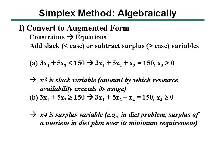
Simplex Method: Algebraically I) Convert to Augmented Form Constraints Equations Add slack ( case) or subtract surplus ( case) variables (a) 3 x 1 + 5 x 2 150 3 x 1 + 5 x 2 + x 3 = 150, x 3 0 à x 3 is slack variable (amount by which resource availability exceeds its usage) (b) 3 x 1 + 5 x 2 150 3 x 1 + 5 x 2 – x 4 = 150, x 4 0 à x 4 is surplus variable (e. g. , in diet problem, surplus of a nutrient in diet plan over its minimum requirement)

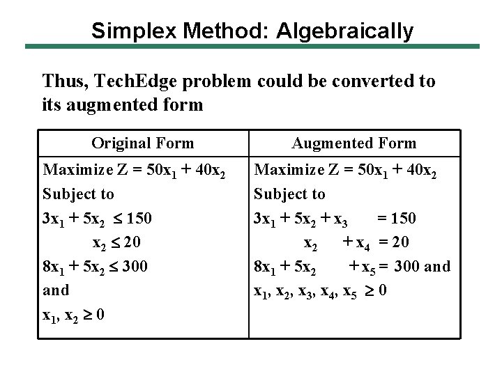
Simplex Method: Algebraically Thus, Tech. Edge problem could be converted to its augmented form Original Form Maximize Z = 50 x 1 + 40 x 2 Subject to 3 x 1 + 5 x 2 150 x 2 20 8 x 1 + 5 x 2 300 and x 1, x 2 0 Augmented Form Maximize Z = 50 x 1 + 40 x 2 Subject to 3 x 1 + 5 x 2 + x 3 = 150 x 2 + x 4 = 20 8 x 1 + 5 x 2 + x 5 = 300 and x 1, x 2, x 3, x 4, x 5 0

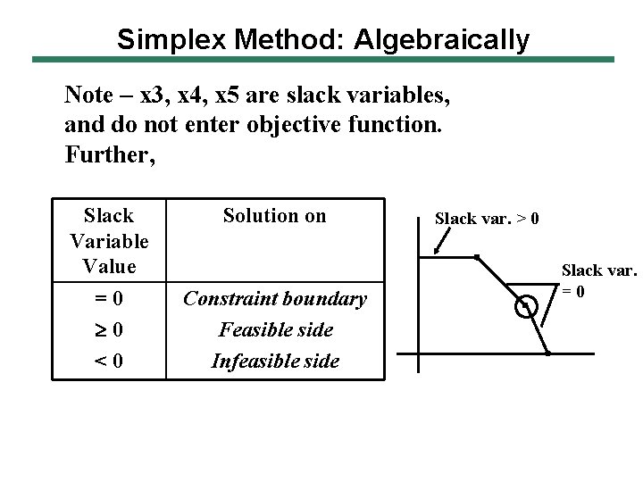
Simplex Method: Algebraically Note – x 3, x 4, x 5 are slack variables, and do not enter objective function. Further, Slack Variable Value Solution on =0 0 <0 Constraint boundary Feasible side Infeasible side Slack var. > 0 Slack var. =0

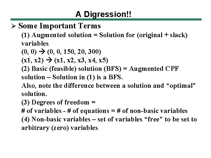
A Digression!! Ø Some Important Terms (1) Augmented solution = Solution for (original + slack) variables (0, 0) (0, 0, 150, 20, 300) (x 1, x 2) (x 1, x 2, x 3, x 4, x 5) (2) Basic (feasible) solution (BFS) = Augmented CPF solution – Solution in (1) is a BFS. Also, note the difference between a solution and “optimal” solution. (3) Degrees of freedom = # of variables - # of equations = # of non-basic variables (4) Non-basic variables – set of variables “free” to be set to arbitrary (zero) variables

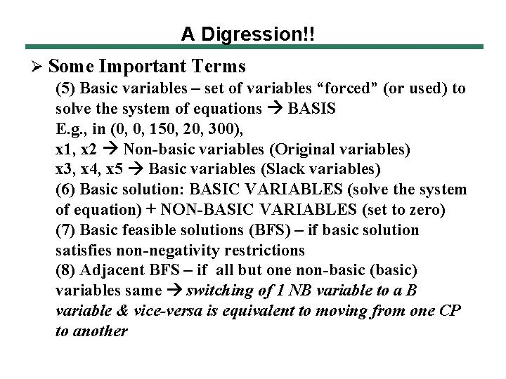
A Digression!! Ø Some Important Terms (5) Basic variables – set of variables “forced” (or used) to solve the system of equations BASIS E. g. , in (0, 0, 150, 20, 300), x 1, x 2 Non-basic variables (Original variables) x 3, x 4, x 5 Basic variables (Slack variables) (6) Basic solution: BASIC VARIABLES (solve the system of equation) + NON-BASIC VARIABLES (set to zero) (7) Basic feasible solutions (BFS) – if basic solution satisfies non-negativity restrictions (8) Adjacent BFS – if all but one non-basic (basic) variables same switching of 1 NB variable to a B variable & vice-versa is equivalent to moving from one CP to another

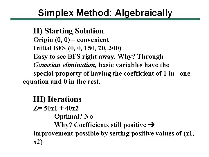
Simplex Method: Algebraically II) Starting Solution Origin (0, 0) – convenient Initial BFS (0, 0, 150, 20, 300) Easy to see BFS right away. Why? Through Gaussian elimination, basic variables have the special property of having the coefficient of 1 in one equation and 0 in the rest. III) Iterations Z= 50 x 1 + 40 x 2 Optimal? No Why? Coefficients still positive improvement possible by setting positive values of (x 1, x 2)

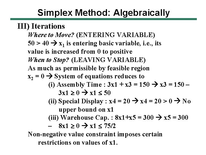
Simplex Method: Algebraically III) Iterations Where to Move? (ENTERING VARIABLE) 50 > 40 x 1 is entering basic variable, i. e. , its value is increased from 0 to positive When to Stop? (LEAVING VARIABLE) As much as permissible by feasible region x 2 = 0 System of equations reduces to (i) Assembly Time : 3 x 1 + x 3 = 150 – 3 x 1 0 x 1 50 (ii) Special Display : x 4 = 20 > 0 No upper bound on x 1 (iii) Warehouse Cap. : 8 x 1+x 5 = 300 – 8 x 1 0 x 1 75/2 Non-negative value constraint imposes certain restrictions on values of x 1.

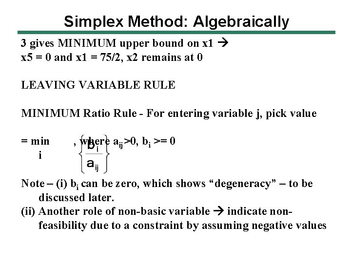
Simplex Method: Algebraically 3 gives MINIMUM upper bound on x 1 x 5 = 0 and x 1 = 75/2, x 2 remains at 0 LEAVING VARIABLE RULE MINIMUM Ratio Rule - For entering variable j, pick value = min i , where aij>0, bi >= 0 Note – (i) bi can be zero, which shows “degeneracy” – to be discussed later. (ii) Another role of non-basic variable indicate nonfeasibility due to a constraint by assuming negative values

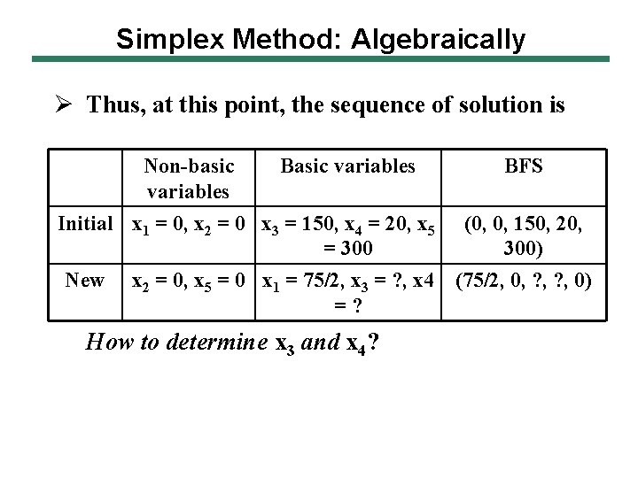
Simplex Method: Algebraically Ø Thus, at this point, the sequence of solution is Non-basic Basic variables BFS variables Initial x 1 = 0, x 2 = 0 x 3 = 150, x 4 = 20, x 5 (0, 0, 150, 20, = 300) New x 2 = 0, x 5 = 0 x 1 = 75/2, x 3 = ? , x 4 (75/2, 0, ? , 0) =? How to determine x 3 and x 4?

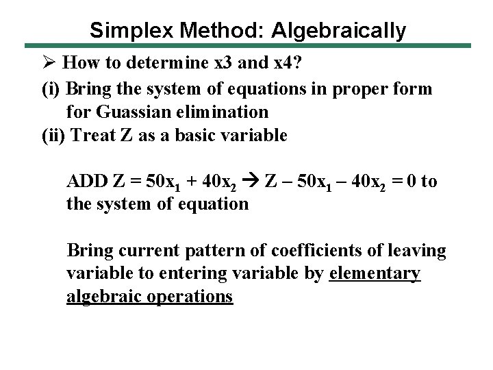
Simplex Method: Algebraically Ø How to determine x 3 and x 4? (i) Bring the system of equations in proper form for Guassian elimination (ii) Treat Z as a basic variable ADD Z = 50 x 1 + 40 x 2 Z – 50 x 1 – 40 x 2 = 0 to the system of equation Bring current pattern of coefficients of leaving variable to entering variable by elementary algebraic operations

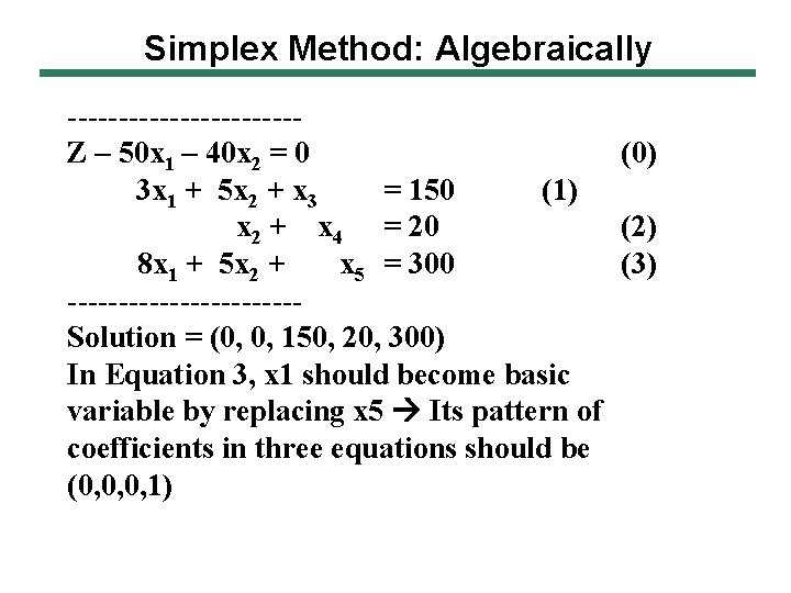
Simplex Method: Algebraically -----------Z – 50 x 1 – 40 x 2 = 0 (0) 3 x 1 + 5 x 2 + x 3 = 150 (1) x 2 + x 4 = 20 (2) 8 x 1 + 5 x 2 + x 5 = 300 (3) -----------Solution = (0, 0, 150, 20, 300) In Equation 3, x 1 should become basic variable by replacing x 5 Its pattern of coefficients in three equations should be (0, 0, 0, 1)

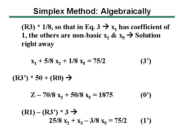
Simplex Method: Algebraically (R 3) * 1/8, so that in Eq. 3 x 1 has coefficient of 1, the others are non-basic x 2 & x 5 Solution right away x 1 + 5/8 x 2 + 1/8 x 5 = 75/2 (3’) (R 3’) * 50 + (R 0) Z – 70/8 x 2 + 50/8 x 5 = 1875 (R 1) – (R 3’) * 3 25/8 x 2 + x 3 – 3/8 x 5 = 75/2 (0’) (1’)

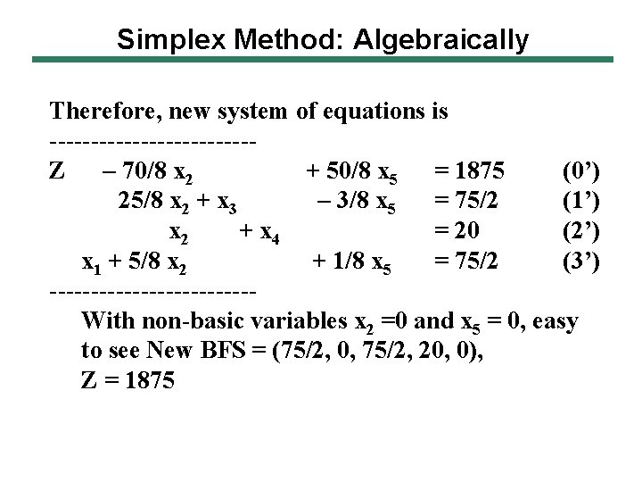
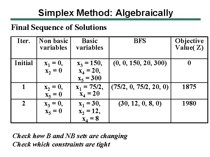
Simplex Method: Algebraically Therefore, new system of equations is ------------Z – 70/8 x 2 + 50/8 x 5 = 1875 (0’) 25/8 x 2 + x 3 – 3/8 x 5 = 75/2 (1’) x 2 + x 4 = 20 (2’) x 1 + 5/8 x 2 + 1/8 x 5 = 75/2 (3’) ------------With non-basic variables x 2 =0 and x 5 = 0, easy to see New BFS = (75/2, 0, 75/2, 20, 0), Z = 1875

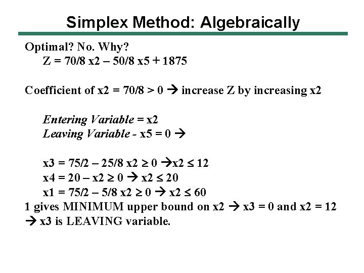
Simplex Method: Algebraically Optimal? No. Why? Z = 70/8 x 2 – 50/8 x 5 + 1875 Coefficient of x 2 = 70/8 > 0 increase Z by increasing x 2 Entering Variable = x 2 Leaving Variable - x 5 = 0 x 3 = 75/2 – 25/8 x 2 0 x 2 12 x 4 = 20 – x 2 0 x 2 20 x 1 = 75/2 – 5/8 x 2 0 x 2 60 1 gives MINIMUM upper bound on x 2 x 3 = 0 and x 2 = 12 x 3 is LEAVING variable.

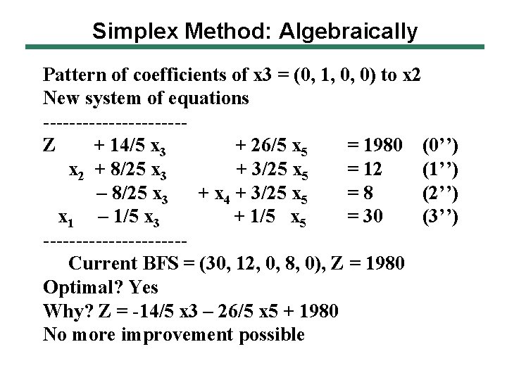
Simplex Method: Algebraically Pattern of coefficients of x 3 = (0, 1, 0, 0) to x 2 New system of equations -----------Z + 14/5 x 3 + 26/5 x 5 = 1980 (0’’) x 2 + 8/25 x 3 + 3/25 x 5 = 12 (1’’) – 8/25 x 3 + x 4 + 3/25 x 5 =8 (2’’) x 1 – 1/5 x 3 + 1/5 x 5 = 30 (3’’) -----------Current BFS = (30, 12, 0, 8, 0), Z = 1980 Optimal? Yes Why? Z = -14/5 x 3 – 26/5 x 5 + 1980 No more improvement possible

Simplex Method: Algebraically Final Sequence of Solutions Iter. Non basic variables BFS Objective Value( Z) Initial x 1 = 0, x 2 = 0 (0, 0, 150, 20, 300) 0 1 x 2 = 0, x 5 = 0 x 3 = 150, x 4 = 20, x 5 = 300 x 1 = 75/2, x 4 = 20 x 1 = 30, x 2 = 12, x 4 = 8 (75/2, 0, 75/2, 20, 0) 1875 (30, 12, 0, 8, 0) 1980 2 Check how B and NB sets are changing Check which constraints are tight

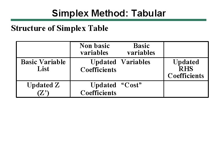
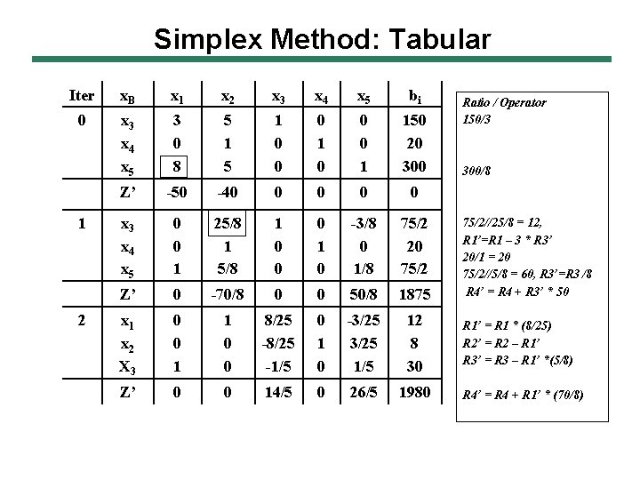
Simplex Method: Tabular Structure of Simplex Table Basic Variable List Updated Z (Z’) Non basic Basic variables Updated Variables Coefficients Updated “Cost” Coefficients Updated RHS Coefficients

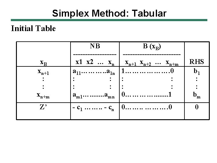
Simplex Method: Tabular Initial Table x. B xn+1 : : xn+m Z’ NB ---------x 1 x 2 … xn a 11………. . a 1 n : : am 1…. . . . amn B (x. B) ------------xn+1 xn+2 … xn+m 1………………. 0 : : 0…………. . . . 1 - c 1 ……. . - cn 0……. . ………. 0 RHS b 1 : : bm 0

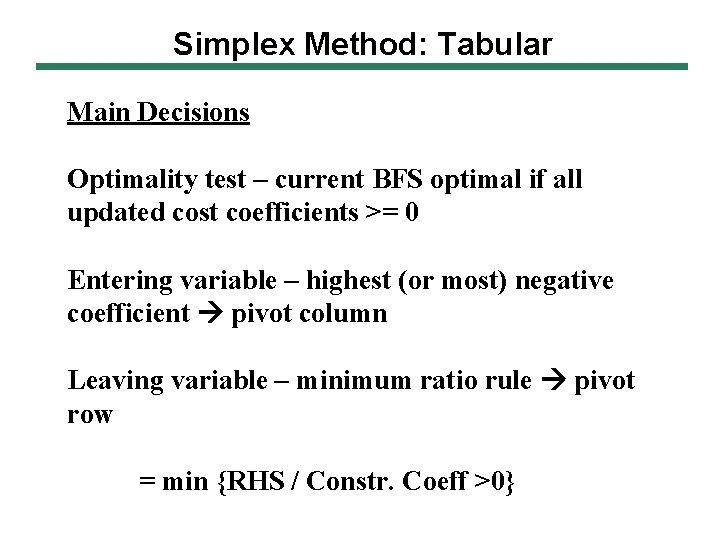
Simplex Method: Tabular Main Decisions Optimality test – current BFS optimal if all updated cost coefficients >= 0 Entering variable – highest (or most) negative coefficient pivot column Leaving variable – minimum ratio rule pivot row = min {RHS / Constr. Coeff >0}

Simplex Method: Tabular Iter x. B x 1 x 2 x 3 x 4 x 5 bi 0 x 3 x 4 x 5 3 0 8 5 1 0 0 0 1 150 20 300 Z’ -50 -40 0 0 x 3 x 4 x 5 0 0 1 25/8 1 0 0 0 1 0 -3/8 0 1/8 75/2 20 75/2 Z’ 0 -70/8 0 0 50/8 1875 x 1 x 2 X 3 0 0 1 1 0 0 8/25 -1/5 0 1 0 -3/25 1/5 12 8 30 Z’ 0 0 14/5 0 26/5 1980 1 2 Ratio / Operator 150/3 300/8 75/2//25/8 = 12, R 1’=R 1 – 3 * R 3’ 20/1 = 20 75/2//5/8 = 60, R 3’=R 3 /8 R 4’ = R 4 + R 3’ * 50 R 1’ = R 1 * (8/25) R 2’ = R 2 – R 1’ R 3’ = R 3 – R 1’ *(5/8) R 4’ = R 4 + R 1’ * (70/8)

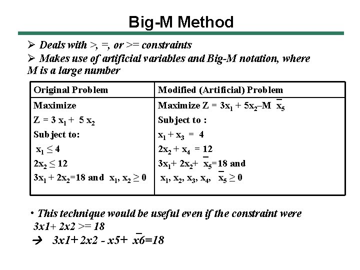
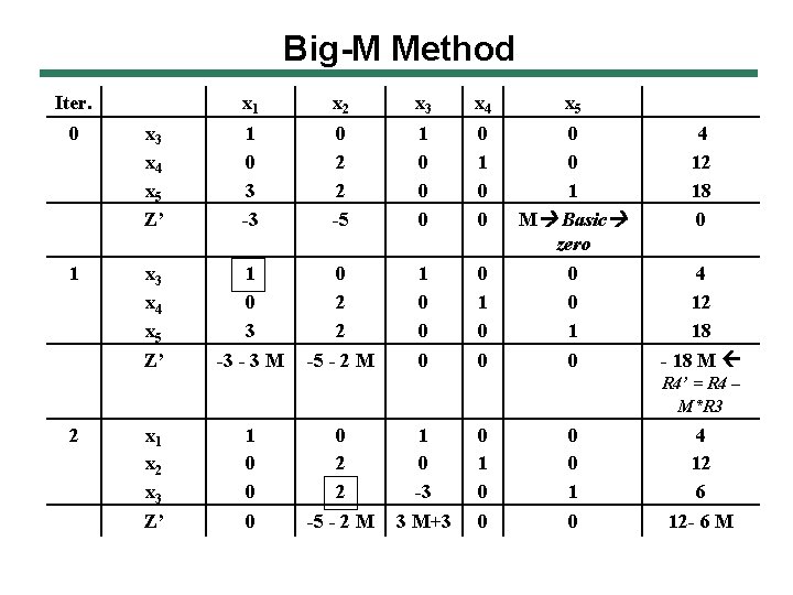
Big-M Method Ø Deals with >, =, or >= constraints Ø Makes use of artificial variables and Big-M notation, where M is a large number Original Problem Modified (Artificial) Problem Maximize Z = 3 x 1 + 5 x 2 Subject to: x 1 ≤ 4 2 x 2 ≤ 12 3 x 1 + 2 x 2=18 and x 1, x 2 ≥ 0 Maximize Z = 3 x 1 + 5 x 2–M x 5 Subject to : x 1 + x 3 = 4 2 x 2 + x 4 = 12 3 x 1+ 2 x 2+ x 5=18 and x 1, x 2, x 3, x 4, x 5 ≥ 0 • This technique would be useful even if the constraint were 3 x 1+ 2 x 2 >= 18 3 x 1+ 2 x 2 - x 5+ x 6=18

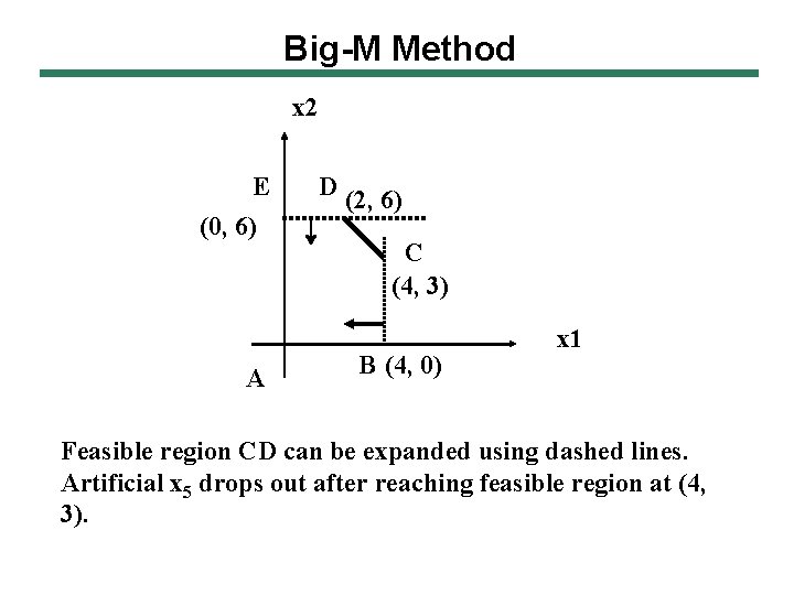
Big-M Method x 2 E (0, 6) A D (2, 6) C (4, 3) B (4, 0) x 1 Feasible region CD can be expanded using dashed lines. Artificial x 5 drops out after reaching feasible region at (4, 3).

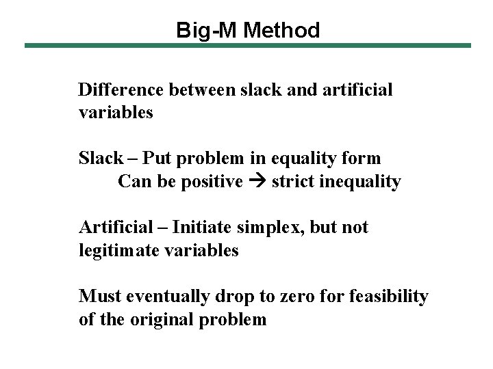
Big-M Method Difference between slack and artificial variables Slack – Put problem in equality form Can be positive strict inequality Artificial – Initiate simplex, but not legitimate variables Must eventually drop to zero for feasibility of the original problem

Big-M Method Iter. x 1 x 2 x 3 x 4 x 5 0 x 3 x 4 x 5 Z’ 1 0 3 -3 0 2 2 -5 1 0 0 0 0 1 M Basic zero 4 12 18 0 1 x 3 x 4 x 5 Z’ 1 0 3 -3 - 3 M 0 2 2 -5 - 2 M 1 0 0 0 0 1 0 4 12 18 - 18 M R 4’ = R 4 – M*R 3 2 x 1 x 2 x 3 Z’ 1 0 0 2 2 -5 - 2 M 1 0 -3 3 M+3 0 1 0 4 12 6 12 - 6 M

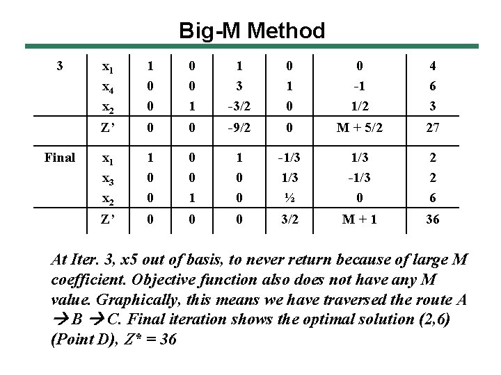
Big-M Method 3 Final x 1 x 4 x 2 1 0 0 1 1 3 -3/2 0 1 0 0 -1 1/2 4 6 3 Z’ 0 0 -9/2 0 M + 5/2 27 x 1 x 3 x 2 1 0 0 1 1 0 0 -1/3 ½ 1/3 -1/3 0 2 2 6 Z’ 0 0 0 3/2 M+1 36 At Iter. 3, x 5 out of basis, to never return because of large M coefficient. Objective function also does not have any M value. Graphically, this means we have traversed the route A B C. Final iteration shows the optimal solution (2, 6) (Point D), Z* = 36

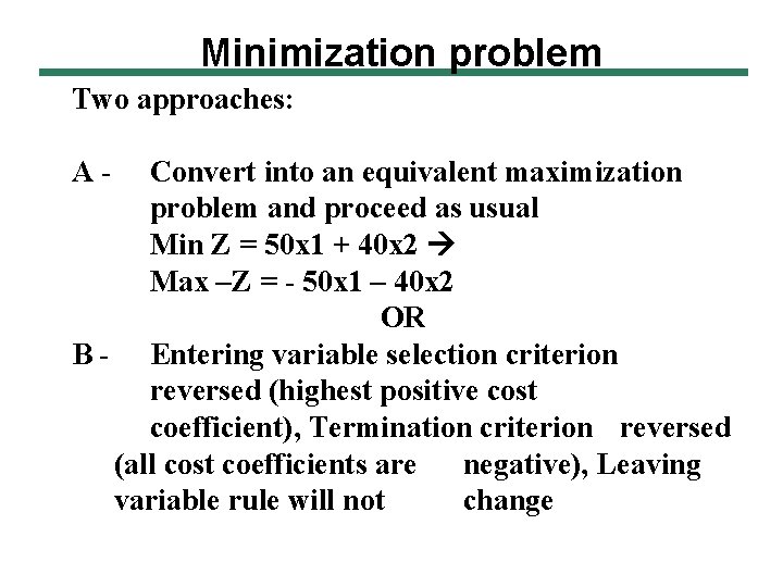
Minimization problem Two approaches: A- Convert into an equivalent maximization problem and proceed as usual Min Z = 50 x 1 + 40 x 2 Max –Z = - 50 x 1 – 40 x 2 OR B - Entering variable selection criterion reversed (highest positive cost coefficient), Termination criterion reversed (all cost coefficients are negative), Leaving variable rule will not change

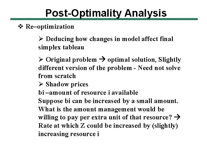
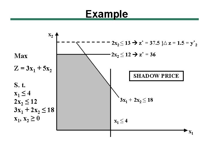
Post-Optimality Analysis v Re–optimization Ø Deducing how changes in model affect final simplex tableau Ø Original problem optimal solution, Slightly different version of the problem - Need not solve from scratch Ø Shadow prices bi –amount of resource i available Suppose bi can be increased by a small amount. What is the amount management would be willing to pay per extra unit of that resource? Rate at which Z could be increased by (slightly) increasing resource i

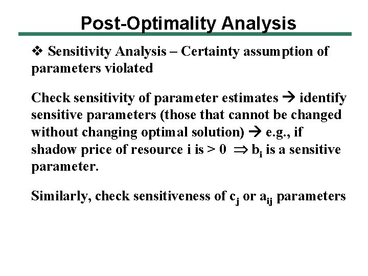
Post-Optimality Analysis v Sensitivity Analysis – Certainty assumption of parameters violated Check sensitivity of parameter estimates identify sensitive parameters (those that cannot be changed without changing optimal solution) e. g. , if shadow price of resource i is > 0 bi is a sensitive parameter. Similarly, check sensitiveness of cj or aij parameters

Example x 2 2 x 2 ≤ 13 z* = 37. 5 }∆ z = 1. 5 = y*2 Max 2 x 2 ≤ 12 z* = 36 Z = 3 x 1 + 5 x 2 S. t. x 1 ≤ 4 2 x 2 ≤ 12 3 x 1 + 2 x 2 ≤ 18 x 1, x 2 ≥ 0 SHADOW PRICE 3 x 1 + 2 x 2 ≤ 18 x 1 ≤ 4 x 1

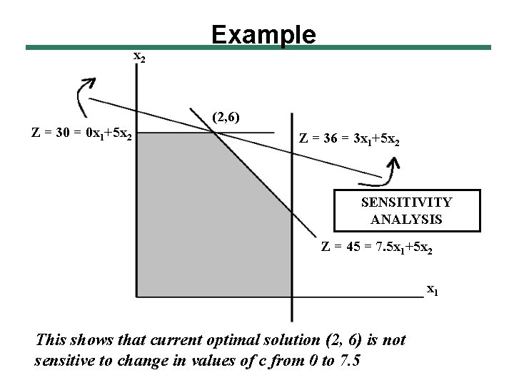
x 2 Z = 30 = 0 x 1+5 x 2 Example (2, 6) Z = 36 = 3 x 1+5 x 2 SENSITIVITY ANALYSIS Z = 45 = 7. 5 x 1+5 x 2 x 1 This shows that current optimal solution (2, 6) is not sensitive to change in values of c from 0 to 7. 5

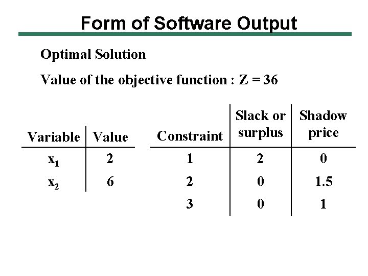
Form of Software Output Optimal Solution Value of the objective function : Z = 36 Variable Value x 1 2 x 2 6 Slack or Shadow price Constraint surplus 1 2 0 1. 5 3 0 1

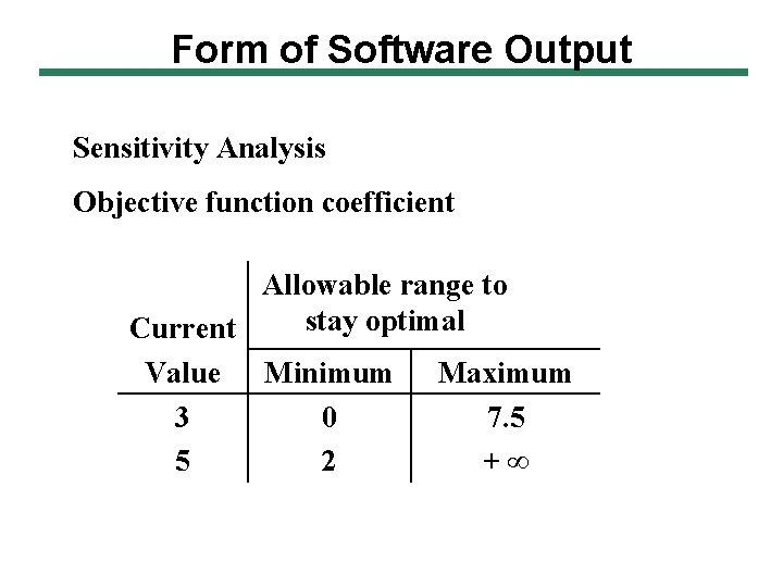
Form of Software Output Sensitivity Analysis Objective function coefficient Allowable range to stay optimal Current Value Minimum Maximum 3 0 7. 5 5 2 +∞

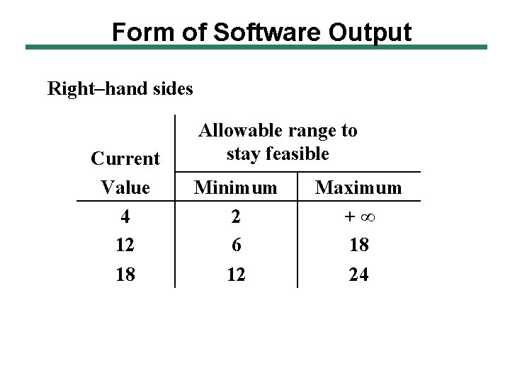
Form of Software Output Right–hand sides Current Value 4 12 18 Allowable range to stay feasible Minimum 2 6 12 Maximum +∞ 18 24

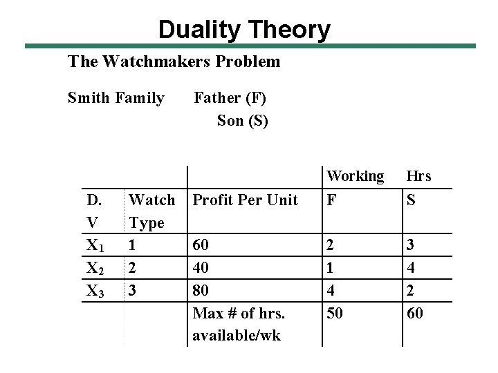
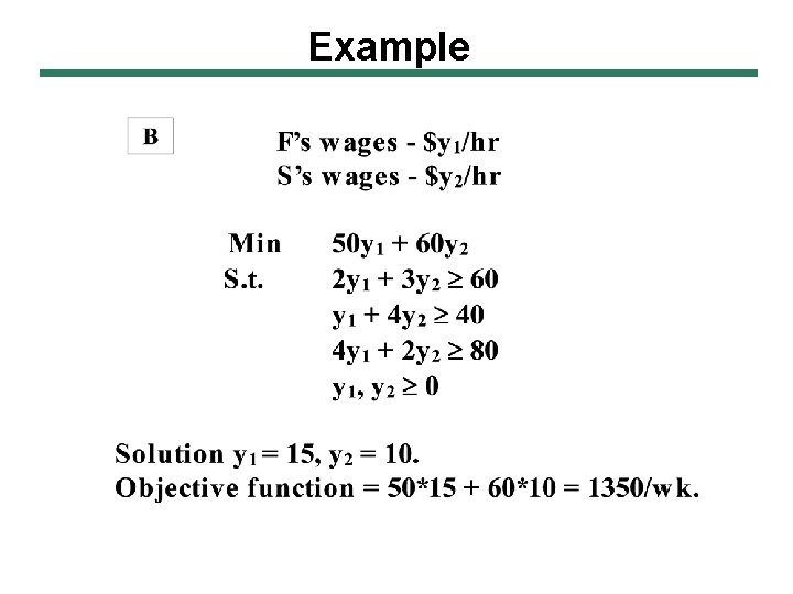
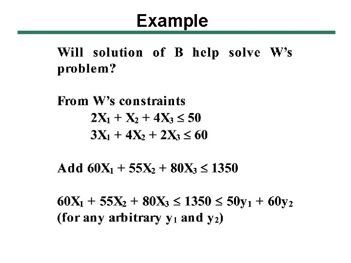
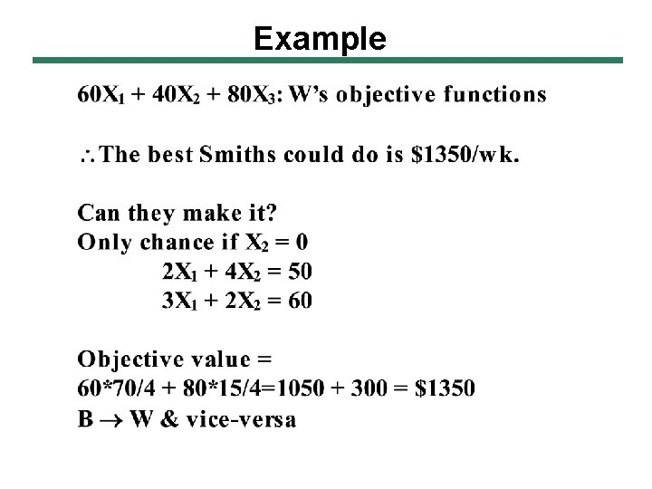
Duality Theory The Watchmakers Problem Smith Family D. V X 1 X 2 X 3 Watch Type 1 2 3 Father (F) Son (S) Working Hrs Profit Per Unit F S 60 40 80 Max # of hrs. available/wk 2 1 4 50 3 4 2 60

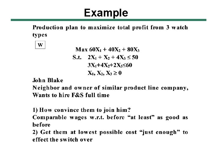
Example

Example

Example

Example

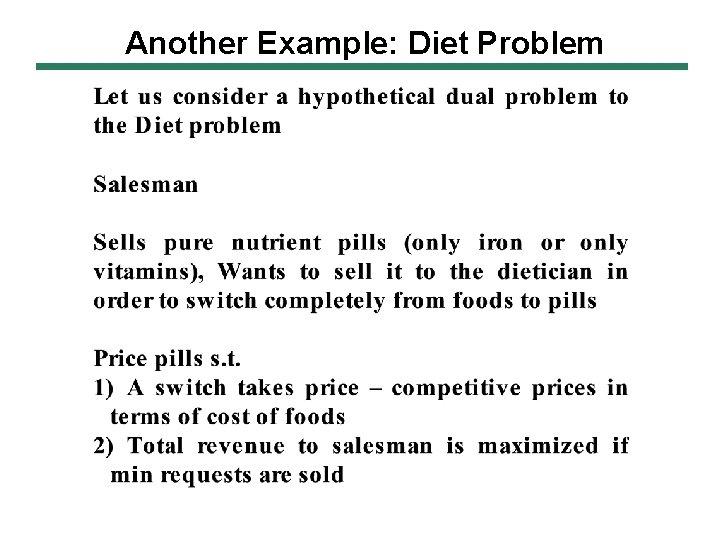
Another Example: Diet Problem

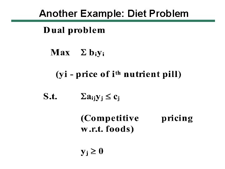
Another Example: Diet Problem

Another Example: Diet Problem

How to get D from P? ?

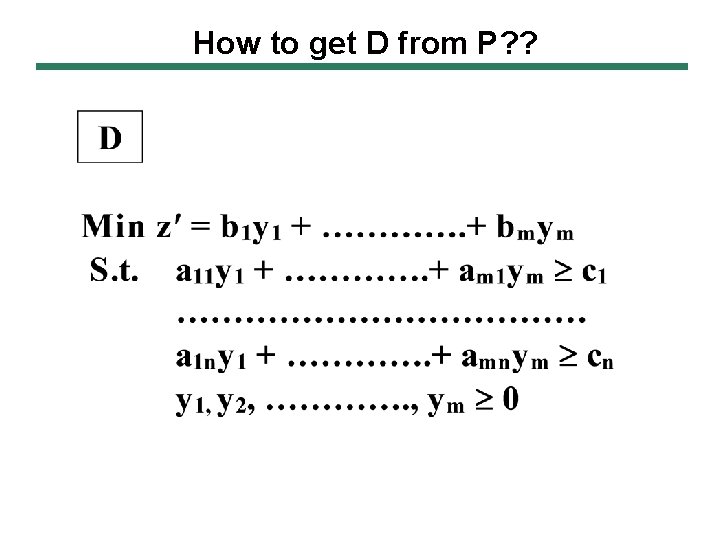
How to get D from P? ?

Summary of P – D Relations

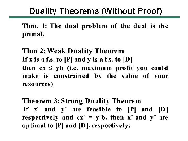
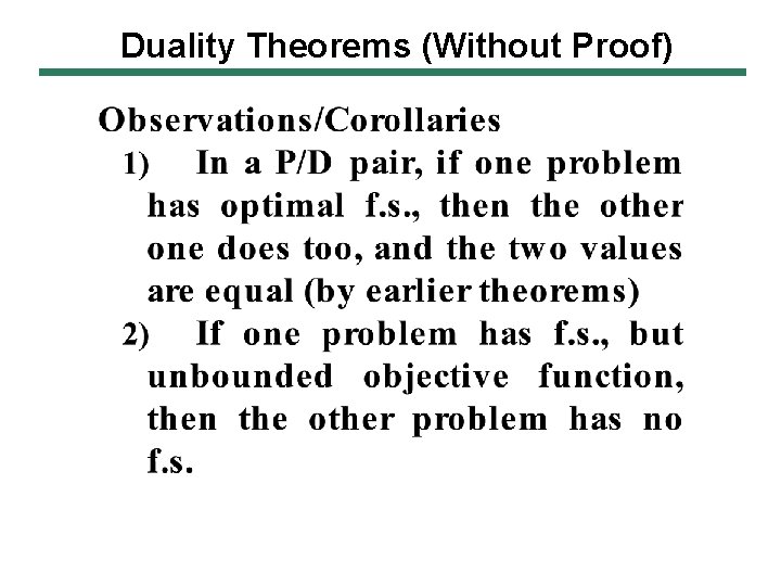
Duality Theorems (Without Proof)

Duality Theorems (Without Proof)

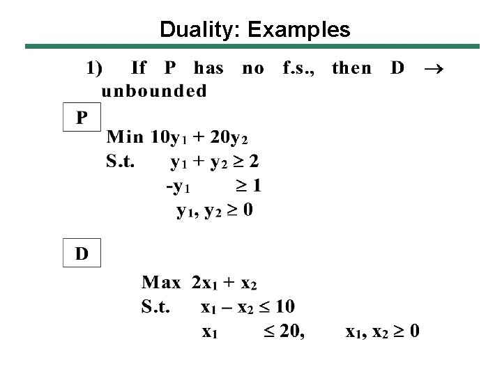
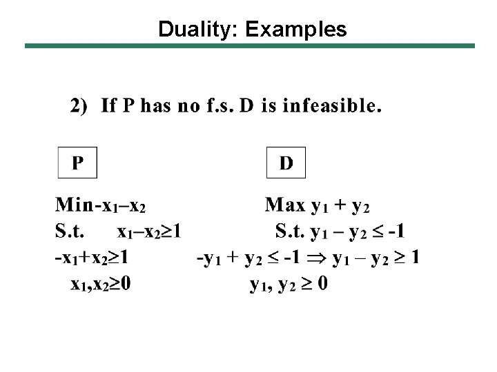
Duality: Examples

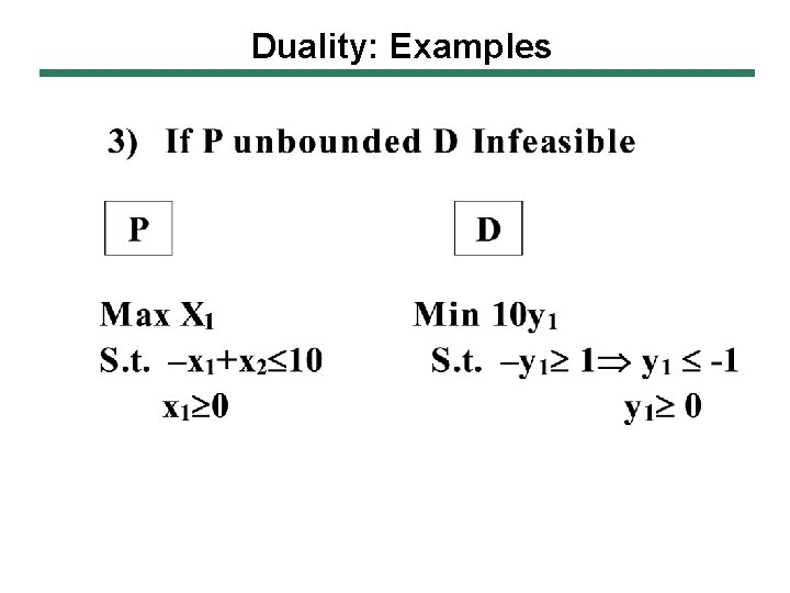
Duality: Examples

Duality: Examples

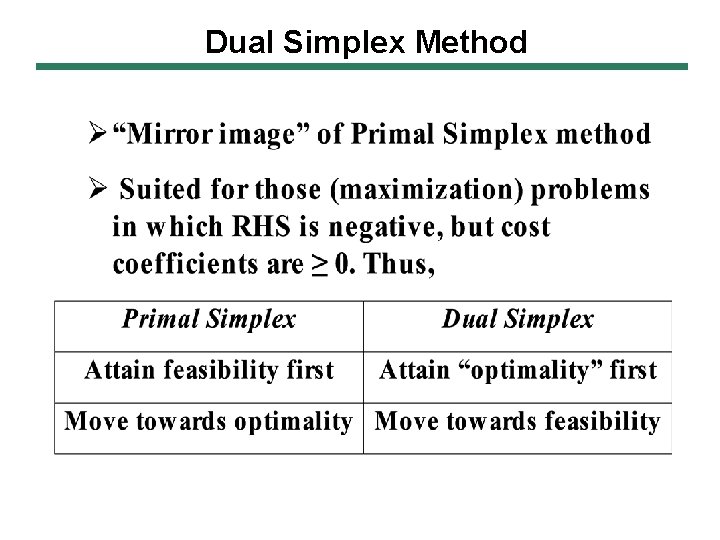
Dual Simplex Method

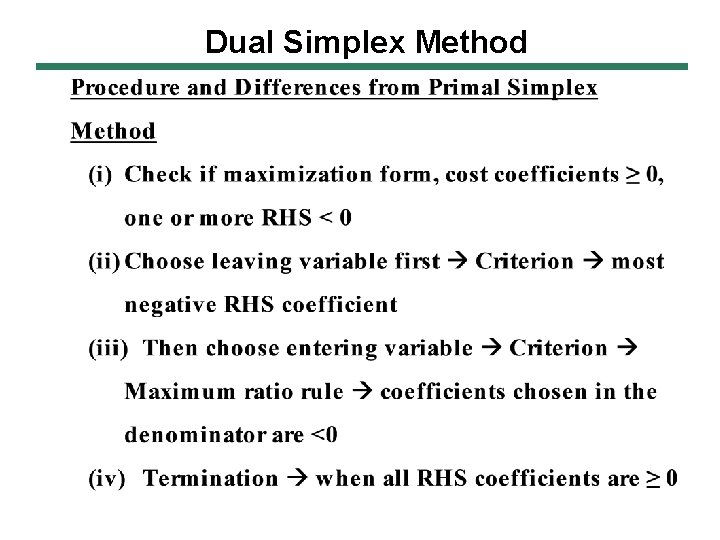
Dual Simplex Method

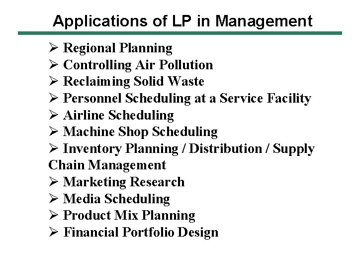
Applications of LP in Management Ø Regional Planning Ø Controlling Air Pollution Ø Reclaiming Solid Waste Ø Personnel Scheduling at a Service Facility Ø Airline Scheduling Ø Machine Shop Scheduling Ø Inventory Planning / Distribution / Supply Chain Management Ø Marketing Research Ø Media Scheduling Ø Product Mix Planning Ø Financial Portfolio Design