Linear models with different types of data Estimate

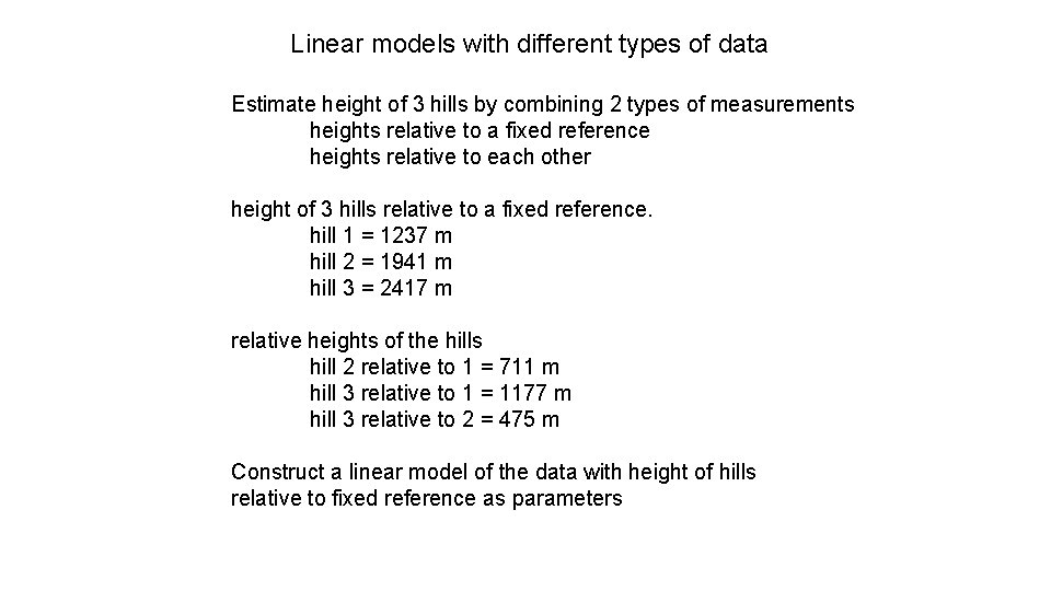
Linear models with different types of data Estimate height of 3 hills by combining 2 types of measurements heights relative to a fixed reference heights relative to each other height of 3 hills relative to a fixed reference. hill 1 = 1237 m hill 2 = 1941 m hill 3 = 2417 m relative heights of the hills hill 2 relative to 1 = 711 m hill 3 relative to 1 = 1177 m hill 3 relative to 2 = 475 m Construct a linear model of the data with height of hills relative to fixed reference as parameters

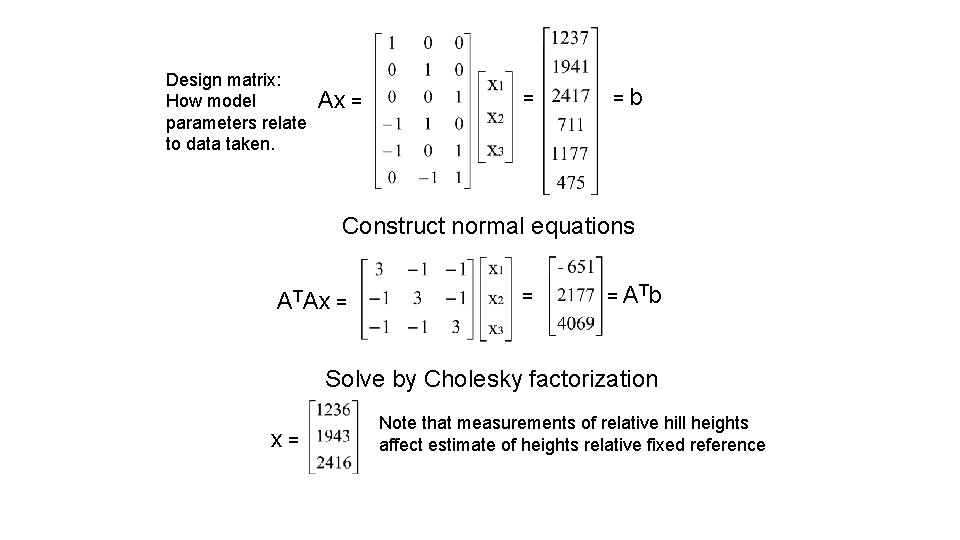
Design matrix: How model parameters relate to data taken. Ax = = =b Construct normal equations ATAx = = = A Tb Solve by Cholesky factorization x= Note that measurements of relative hill heights affect estimate of heights relative fixed reference

QR factorization of non-square matrices Alternative to Normal Equation

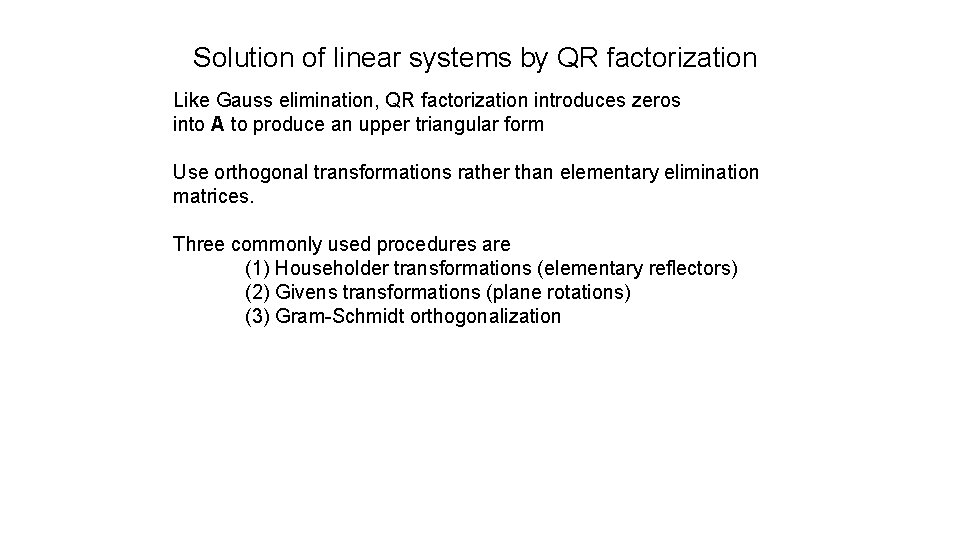
Solution of linear systems by QR factorization Like Gauss elimination, QR factorization introduces zeros into A to produce an upper triangular form Use orthogonal transformations rather than elementary elimination matrices. Three commonly used procedures are (1) Householder transformations (elementary reflectors) (2) Givens transformations (plane rotations) (3) Gram-Schmidt orthogonalization

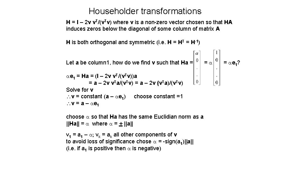
Householder transformations H = I – 2 v v. T/(v. Tv) where v is a non-zero vector chosen so that HA induces zeros below the diagonal of some column of matrix A H is both orthogonal and symmetric (i. e. H = HT = H-1) Let a be column 1, how do we find v such that Ha = ae 1 = Ha = (I – 2 v v. T/(v. Tv))a = a – 2 v v. Ta/(v. Tv) = a – 2 v (v. Ta)/(v. Tv) Solve for v v = constant (a – ae 1) choose constant =1 v = a – ae 1 choose a so that Ha has the same Euclidian norm as a ||Ha|| = a where a = + ||a|| v 1 = a 1 – a; vk = ak all other components of v to avoid loss of significance chose a = -sign(a 1)||a|| (i. e. if a 1 is positive then a is negative) =a = ae 1?

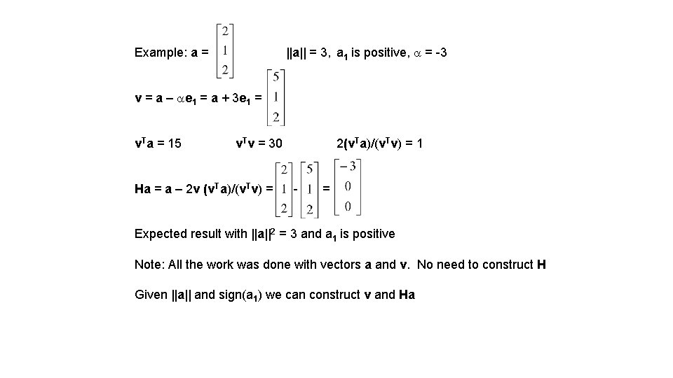
||a|| = 3, a 1 is positive, a = -3 Example: a = v = a – ae 1 = a + 3 e 1 = v. Ta = 15 v. Tv = 30 Ha = a – 2 v (v. Ta)/(v. Tv) = 2(v. Ta)/(v. Tv) = 1 - = Expected result with ||a||2 = 3 and a 1 is positive Note: All the work was done with vectors a and v. No need to construct H Given ||a|| and sign(a 1) we can construct v and Ha

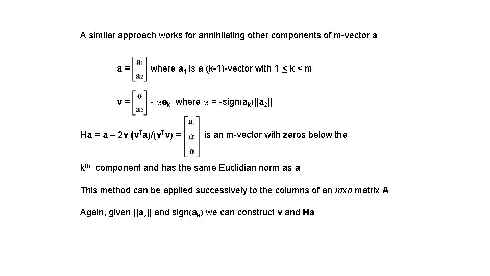
A similar approach works for annihilating other components of m-vector a a= where a 1 is a (k-1)-vector with 1 < k < m v= - aek where a = -sign(ak)||a 2|| Ha = a – 2 v (v. Ta)/(v. Tv) = is an m-vector with zeros below the kth component and has the same Euclidian norm as a This method can be applied successively to the columns of an mxn matrix A Again, given ||a 2|| and sign(ak) we can construct v and Ha

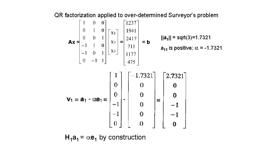
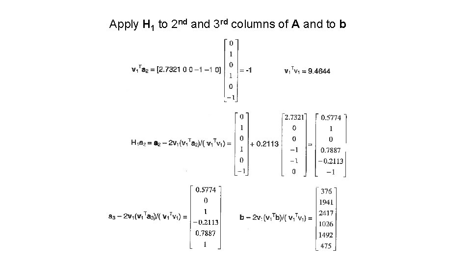
QR factorization applied to over-determined Surveyor’s problem Ax = = =b H 1 a 1 = ae 1 by construction ||a 1|| = sqrt(3)=1. 7321 a 11 is positive; a = -1. 7321

Apply H 1 to 2 nd and 3 rd columns of A and to b

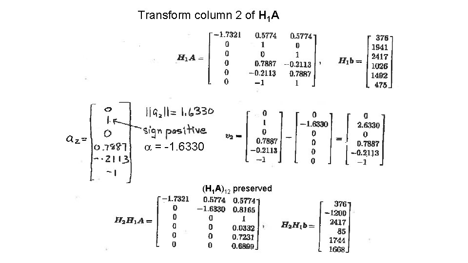
Transform column 2 of H 1 A a = -1. 6330 (H 1 A)12 preserved

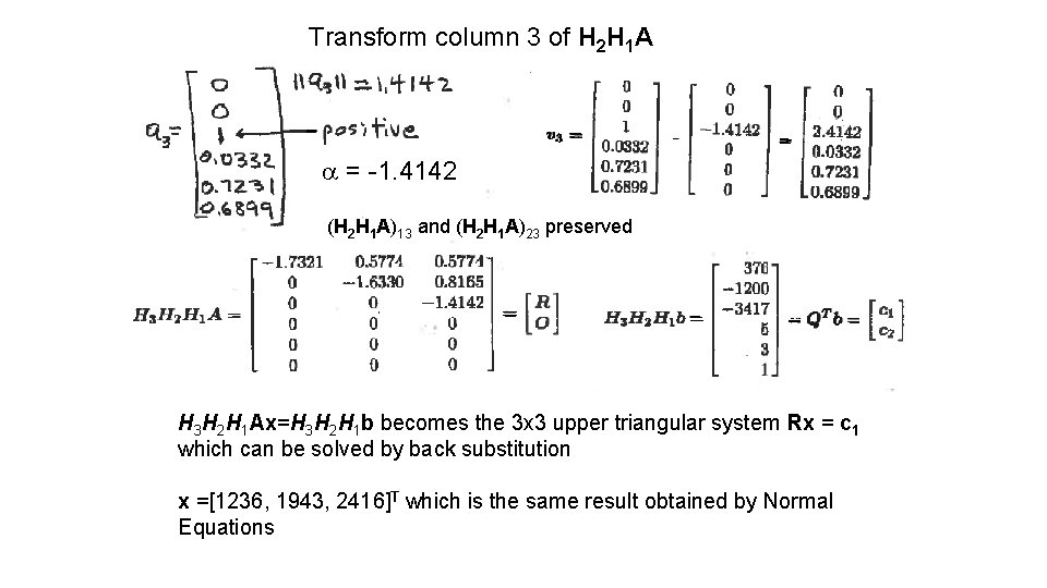
Transform column 3 of H 2 H 1 A a = -1. 4142 (H 2 H 1 A)13 and (H 2 H 1 A)23 preserved H 3 H 2 H 1 Ax=H 3 H 2 H 1 b becomes the 3 x 3 upper triangular system Rx = c 1 which can be solved by back substitution x =[1236, 1943, 2416]T which is the same result obtained by Normal Equations

Application of Mat. Lab’s QR factorization to Linear Least Squares

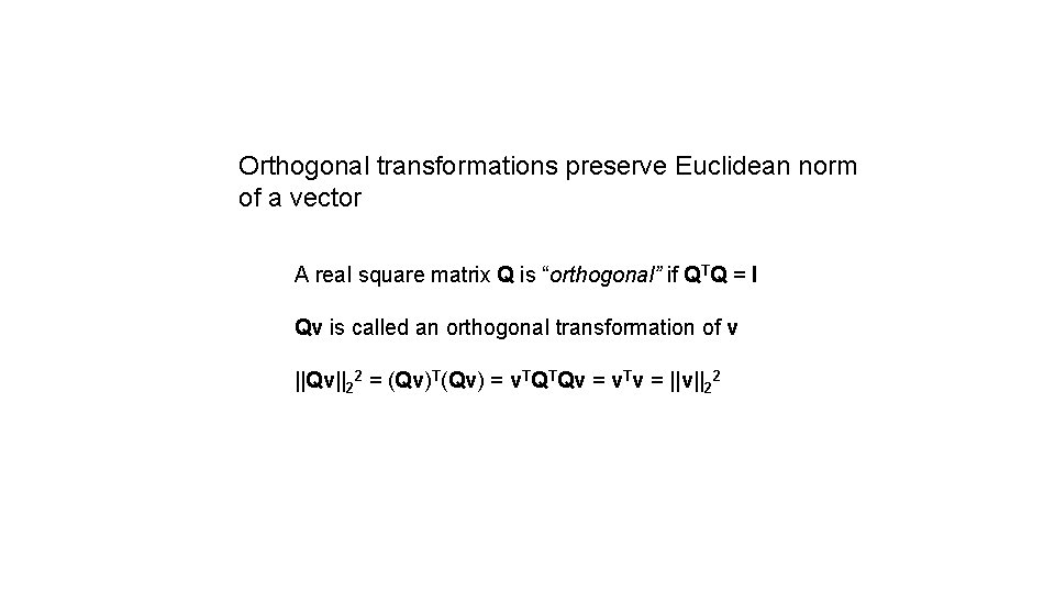
Orthogonal transformations preserve Euclidean norm of a vector A real square matrix Q is “orthogonal” if QTQ = I Qv is called an orthogonal transformation of v ||Qv||22 = (Qv)T(Qv) = v. TQTQv = v. Tv = ||v||22

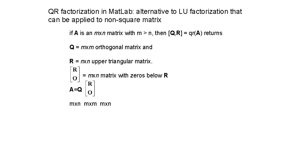
QR factorization in Mat. Lab: alternative to LU factorization that can be applied to non-square matrix if A is an mxn matrix with m > n, then [Q, R] = qr(A) returns Q = mxm orthogonal matrix and R = nxn upper triangular matrix. = mxn matrix with zeros below R A=Q mxn mxm mxn

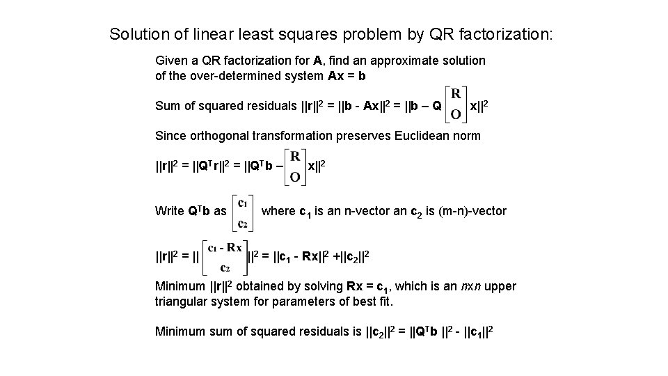
Solution of linear least squares problem by QR factorization: Given a QR factorization for A, find an approximate solution of the over-determined system Ax = b Sum of squared residuals ||r||2 = ||b - Ax||2 = ||b – Q x||2 Since orthogonal transformation preserves Euclidean norm ||r||2 = ||QTb – Write QTb as ||r||2 = || x||2 where c 1 is an n-vector an c 2 is (m-n)-vector ||2 = ||c 1 - Rx||2 +||c 2||2 Minimum ||r||2 obtained by solving Rx = c 1, which is an nxn upper triangular system for parameters of best fit. Minimum sum of squared residuals is ||c 2||2 = ||QTb ||2 - ||c 1||2

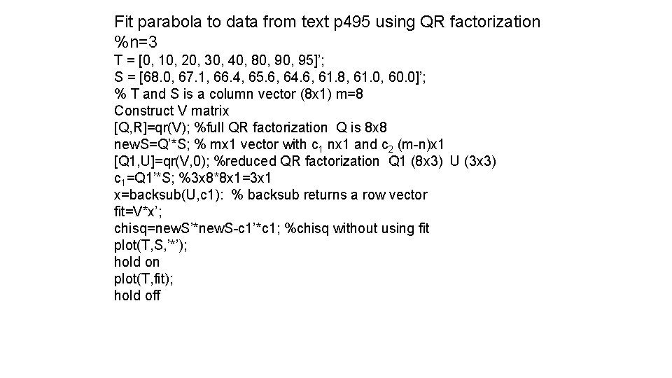
Fit parabola to data from text p 495 using QR factorization %n=3 T = [0, 10, 20, 30, 40, 80, 95]’; S = [68. 0, 67. 1, 66. 4, 65. 6, 64. 6, 61. 8, 61. 0, 60. 0]’; % T and S is a column vector (8 x 1) m=8 Construct V matrix [Q, R]=qr(V); %full QR factorization Q is 8 x 8 new. S=Q’*S; % mx 1 vector with c 1 nx 1 and c 2 (m-n)x 1 [Q 1, U]=qr(V, 0); %reduced QR factorization Q 1 (8 x 3) U (3 x 3) c 1=Q 1’*S; %3 x 8*8 x 1=3 x 1 x=backsub(U, c 1): % backsub returns a row vector fit=V*x’; chisq=new. S’*new. S-c 1’*c 1; %chisq without using fit plot(T, S, ’*’); hold on plot(T, fit); hold off

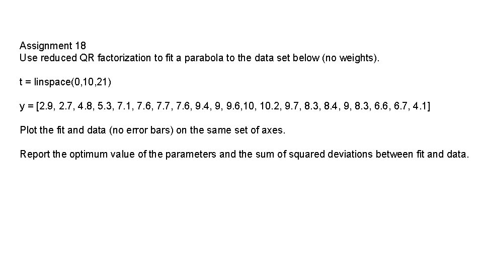
Assignment 18 Use reduced QR factorization to fit a parabola to the data set below (no weights). t = linspace(0, 10, 21) y = [2. 9, 2. 7, 4. 8, 5. 3, 7. 1, 7. 6, 7. 7, 7. 6, 9. 4, 9, 9. 6, 10. 2, 9. 7, 8. 3, 8. 4, 9, 8. 3, 6. 6, 6. 7, 4. 1] Plot the fit and data (no error bars) on the same set of axes. Report the optimum value of the parameters and the sum of squared deviations between fit and data.