Linear Models for Regression CSE 4309 Machine Learning

Linear Models for Regression CSE 4309 – Machine Learning Vassilis Athitsos Computer Science and Engineering Department University of Texas at Arlington 1

The Regression Problem • 2

A Regression Example • circles: training data. • red curve: one possible solution: a line. • green curve: another possible solution: a cubic polynomial. 3

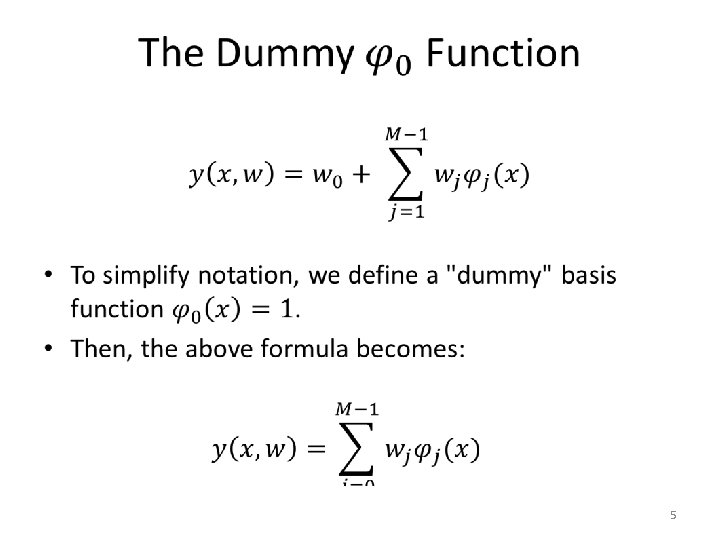
Linear Models for Regression • 4

Dot Product Version • 6

Common Choices for Basis Functions • 7

Common Choices for Basis Functions • 8

Common Choices for Basis Functions • 9

Common Choices for Basis Functions • 10

Common Choices for Basis Functions • 11

Global Versus Local Functions • 12

Linear Versus Nonlinear Functions • A linear function y(x, w) produces an output that depends linearly on both x and w. • Note that polynomial, Gaussian, and sigmoidal basis functions are nonlinear. • If we use nonlinear basis functions, then the regression process produces a function y(x, w) which is: – Linear to w. – Nonlinear to x. • It is important to remember: linear regression can be used to estimate nonlinear functions of x. – It is called linear regression because y is linear to w, NOT because y is linear to x. 13

Solving Regression Problems • There are different methods for solving regression problems. • We will study two approaches: – Least squares: find the weights w that minimize the squared error. – Regularized least squares: find the weights w that minimize the squared error, using some hand-picked regularization parameter λ. 14

The Gaussian Noise Assumption • 15

The Gaussian Noise Assumption • 16

Finding the Most Likely Solution • 17

Finding the Most Likely Solution • 18

Likelihood of the Training Data • 19

Likelihood of the Training Data • 20

Log Likelihood of the Training Data • 21

Log Likelihood of the Training Data 22

Log Likelihood of the Training Data • 23

Log Likelihood and Sum-of-Squares Error • 24

Minimizing Sum-of-Squares Error • 25

Minimizing Sum-of-Squares Error • 26

Minimizing Sum-of-Squares Error • 27

Minimizing Sum-of-Squares Error • 28

Minimizing Sum-of-Squares Error • 29

Minimizing Sum-of-Squares Error • 30

Minimizing Sum-of-Squares Error • 31

Minimizing Sum-of-Squares Error • 32

Minimizing Sum-of-Squares Error • 33

Minimizing Sum-of-Squares Error • 34

Minimizing Sum-of-Squares Error • 35

Minimizing Sum-of-Squares Error • 36

Minimizing Sum-of-Squares Error • 37

Minimizing Sum-of-Squares Error • Transposing both sides 38

Minimizing Sum-of-Squares Error • 39

Minimizing Sum-of-Squares Error • 40

Minimizing Sum-of-Squares Error • 41

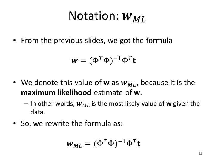
Solving for β • 43

Least Squares Solution - Summary • 44

Numerical Issues • Black circles: training data. • Green curve: true function y(x)=sin(2πx). • Red curve: – Top figure: Fitted 7 -degree polynomial. – Bottom figure: Fitted 8 -degree polynomial. • Do you see anything strange? 45

Numerical Issues • The 8 -degree polynomial fits the data worse than the 7 degree polynomial. • Is this possible? 46

Numerical Issues • The 8 -degree polynomial fits the data worse than the 7 degree polynomial. • Mathematically, this is impossible. • 8 -degree polynomials are a superset of 7 -degree polynomials. • Thus, the best-fitting 8 -degree polynomial cannot fit the data worse than the best-fitting 7 degree polynomial. 47

Numerical Issues • 48

Numerical Issues • Work-around in Matlab: • inv(phi' * phi) leads to the incorrect 8 -degree polynomial fit below. • pinv(phi' * phi) leads to the correct 8 -degree polynomial fit above (almost identical to the 7 -degree result). 49

Sequential Learning • 50

Sequential Learning • 51

Sequential Learning • 52

Sequential Learning - Intuition • 53

Sequential Learning - Intuition • 54

Regularized Least Squares • 55

Solving Regularized Least Squares • 56

Why Use Regularization? • 57

Impact of Parameter λ 58

Impact of Parameter λ 59

Impact of Parameter λ • As the previous figures show: – Low values of λ lead to polynomials whose values fluctuate more and more rapidly. • This can lead to increased overfitting. – High values of λ lead to flatter and flatter polynomials, that look more and more like straight lines. • This can lead to increased underfitting, or not fitting the data sufficiently. 60