Linear model implies a correlation matrix Linear model

Linear model implies a correlation matrix

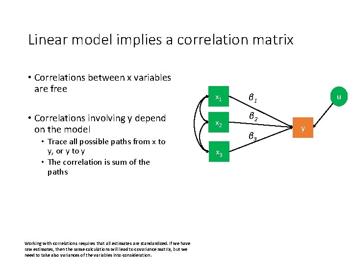
Linear model implies a correlation matrix • Correlations between x variables are free x 1 • Correlations involving y depend on the model x 2 • Trace all possible paths from x to y, or y to y • The correlation is sum of the paths x 3 Working with correlations requires that all estimates are standardized. If we have raw estimates, then the same calculations will lead to covariance matrix, but we need to take also variances of the variables into consideration. u β 1 β 2 β 3 y

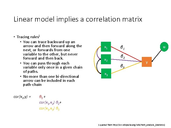
Linear model implies a correlation matrix • Tracing rules 1 • You can trace backward up an arrow and then forward along the next, or forwards from one variable to the other, but never forward and then back. • You can pass through each variable only once in a given chain of paths. • No more than one bi-directional arrow can be included in each path-chain cor(x 1, y) = x 1 x 2 u β 1 β 2 β 3 y x 3 β 1 + cor(x 1, x 2) β 2+ cor(x 1, x 3) β 3 1 quoted from http: //en. wikipedia. org/wiki/Path_analysis_(statistics)

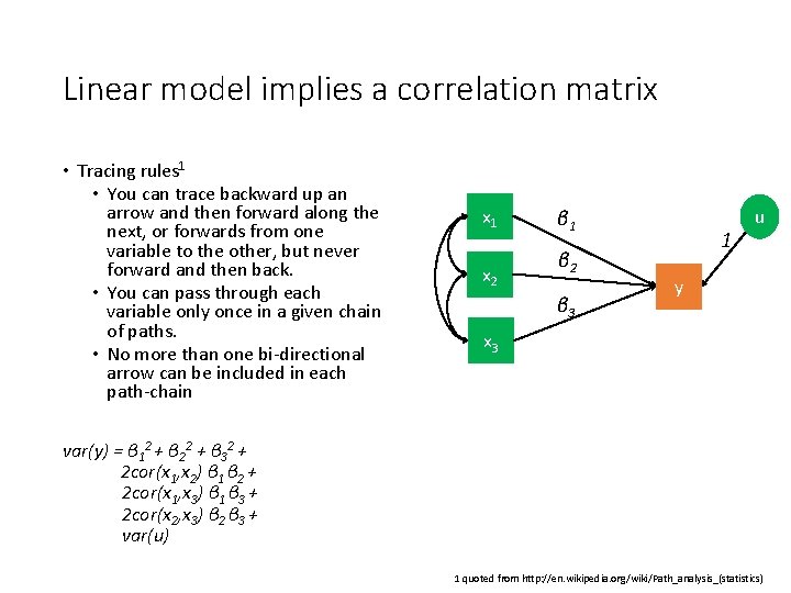
Linear model implies a correlation matrix • Tracing rules 1 • You can trace backward up an arrow and then forward along the next, or forwards from one variable to the other, but never forward and then back. • You can pass through each variable only once in a given chain of paths. • No more than one bi-directional arrow can be included in each path-chain x 1 x 2 β 1 β 2 β 3 1 u y x 3 var(y) = β 12 + β 22 + β 32 + 2 cor(x 1, x 2) β 1 β 2 + 2 cor(x 1, x 3) β 1 β 3 + 2 cor(x 2, x 3) β 2 β 3 + var(u) 1 quoted from http: //en. wikipedia. org/wiki/Path_analysis_(statistics)

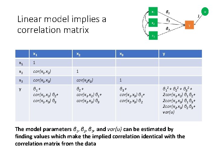
Linear model implies a correlation matrix x 1 x 2 x 3 x 1 1 x 2 cor(x 1, x 2) 1 x 3 cor(x 1, x 3) cor(x 2 x 3) 1 y β 1 + cor(x 1, x 2) β 2+ cor(x 1, x 3) β 3 β 2 + cor(x 1, x 2) β 1+ cor(x 2, x 3) β 3 + cor(x 1, x 3) β 1+ cor(x 2, x 3) β 2 y β 1 2 + β 2 2 + β 3 2 + 2 cor(x 1, x 2) β 1 β 2+ 2 cor(x 1, x 3) β 1 β 3+ 2 cor(x 2, x 3) β 2 β 3+ var(u) The model parameters β 1, β 2, β 3, and var(u) can be estimated by finding values which make the implied correlation identical with the correlation matrix from the data

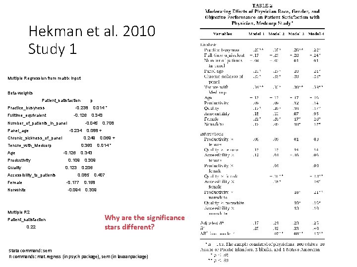
Hekman et al. 2010 Study 1 Multiple Regression from matrix input Beta weights Patient_satisfaction Practice_busyness p -0. 238 Fulltime_equivalent -0. 126 Number_of_patients_in_panel Panel_age -0. 234 0. 360 -0. 126 Quality 0. 014 * 0. 109 0. 309 0. 206 0. 085 0. 407 Female -0. 177 0. 158 Nonwhite -0. 094 0. 309 Multiple R 2 Patient_satisfaction 0. 22 0. 069 + 0. 343 0. 123 Accessibility_to_patients 0. 708 0. 088 + 0. 249 Tenure_with_Medcorp Productivity 0. 343 -0. 045 Chronic_sickness_of_panel Age 0. 014 * Why are the significance stars different? Stata command: sem R commands: mat. regress (in psych package), sem (in lavaanpackage)

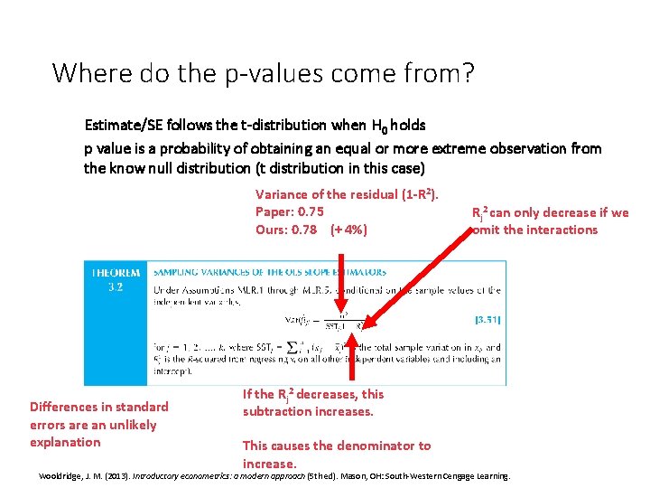
Where do the p-values come from? Estimate/SE follows the t-distribution when H 0 holds p value is a probability of obtaining an equal or more extreme observation from the know null distribution (t distribution in this case) Variance of the residual (1 -R 2). Paper: 0. 75 Ours: 0. 78 (+ 4%) Differences in standard errors are an unlikely explanation Rj 2 can only decrease if we omit the interactions If the Rj 2 decreases, this subtraction increases. This causes the denominator to increase. Wooldridge, J. M. (2013). Introductory econometrics: a modern approach (5 th ed). Mason, OH: South-Western Cengage Learning.

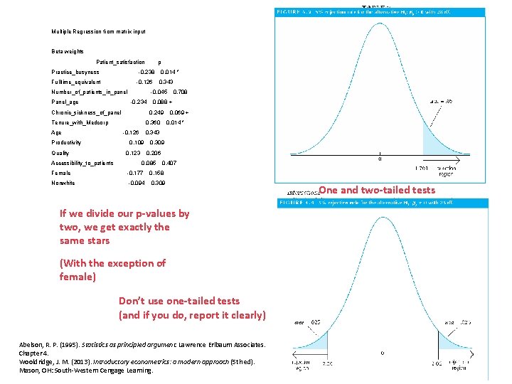
Multiple Regression from matrix input Beta weights Patient_satisfaction Practice_busyness p -0. 238 Fulltime_equivalent -0. 126 Number_of_patients_in_panel Panel_age Quality Accessibility_to_patients 0. 360 -0. 126 0. 708 0. 088 + 0. 249 Tenure_with_Medcorp Productivity 0. 343 -0. 045 -0. 234 Chronic_sickness_of_panel Age 0. 014 * 0. 069 + 0. 014 * 0. 343 0. 109 0. 123 0. 309 0. 206 0. 085 0. 407 Female -0. 177 0. 158 Nonwhite -0. 094 0. 309 If we divide our p-values by two, we get exactly the same stars (With the exception of female) Don’t use one-tailed tests (and if you do, report it clearly) Abelson, R. P. (1995). Statistics as principled argument. Lawrence Erlbaum Associates. Chapter 4. Wooldridge, J. M. (2013). Introductory econometrics: a modern approach (5 th ed). Mason, OH: South-Western Cengage Learning. One and two-tailed tests

Linear model implies a covariance matrix

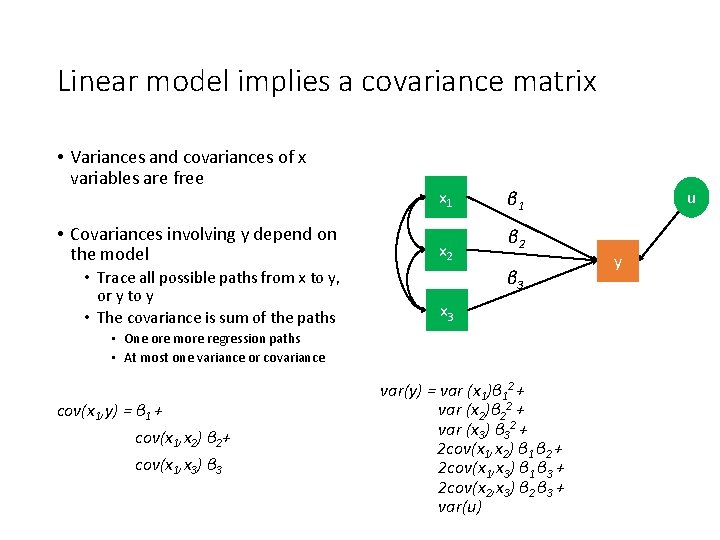
Linear model implies a covariance matrix • Variances and covariances of x variables are free x 1 • Covariances involving y depend on the model x 2 • Trace all possible paths from x to y, or y to y • The covariance is sum of the paths x 3 β 2 β 3 • One ore more regression paths • At most one variance or covariance cov(x 1, y) = β 1 + cov(x 1, x 2) β 2+ cov(x 1, x 3) β 3 u β 1 var(y) = var (x 1)β 12 + var (x 2)β 22 + var (x 3) β 32 + 2 cov(x 1, x 2) β 1 β 2 + 2 cov(x 1, x 3) β 1 β 3 + 2 cov(x 2, x 3) β 2 β 3 + var(u) y

Suppression in regression

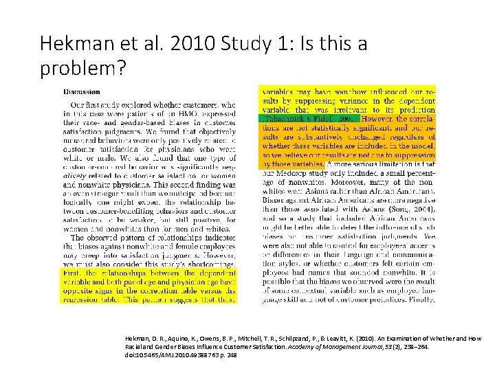
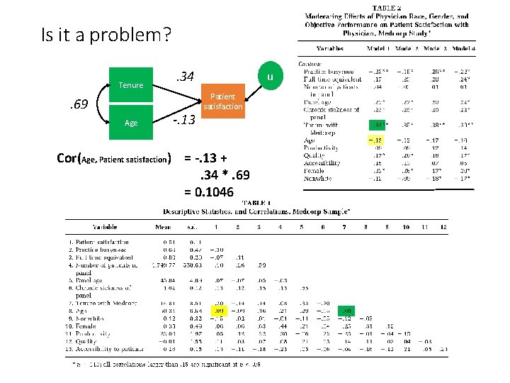
Hekman et al. 2010 Study 1: Is this a problem? Hekman, D. R. , Aquino, K. , Owens, B. P. , Mitchell, T. R. , Schilpzand, P. , & Leavitt, K. (2010). An Examination of Whether and How Racial and Gender Biases Influence Customer Satisfaction. Academy of Management Journal, 53(2), 238– 264. doi: 10. 5465/AMJ. 2010. 49388763 p. 248

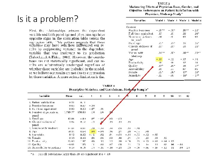
Is it a problem?

Is it a problem? Tenure . 69 Age . 34 -. 13 u Patient satisfaction Cor(Age, Patient satisfaction) = -. 13 +. 34 *. 69 = 0. 1046

Multicollinearity

What does this mean Hekman, D. R. , Aquino, K. , Owens, B. P. , Mitchell, T. R. , Schilpzand, P. , & Leavitt, K. (2010). An Examination of Whether and How Racial and Gender Biases Influence Customer Satisfaction. Academy of Management Journal, 53(2), 238– 264. doi: 10. 5465/AMJ. 2010. 49388763 p. 258

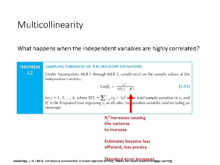
Multicollinearity What happens when the independent variables are highly correlated? Rj 2 increases causing the variance to increase Estimates become less efficient, less precise Standard error increases Wooldridge, J. M. (2013). Introductory econometrics: a modern approach (5 th ed). Mason, OH: South-Western Cengage Learning.

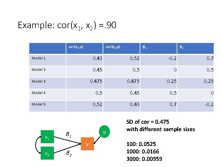
Example: cor(x 1, x 2) =. 90 cor(x 1, y) cor(x 2, y) β 1 β 2 Model 1 0. 43 0. 52 -0. 2 0. 7 Model 2 0. 45 0. 5 0 0. 5 Model 3 0. 475 0. 25 Model 4 0. 5 0. 45 0. 5 0 Model 5 0. 52 0. 43 0. 7 -0. 2 x 1 β 1 x 2 β 2 u y SD of cor = 0. 475 with different sample sizes 100: 0. 0525 1000: 0. 0166 3000: 0. 00959

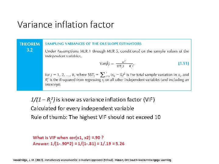
Variance inflation factor 1/(1 – Rj 2) is know as variance inflation factor (VIF) Calculated for every independent variable Rule of thumb: The highest VIF should not exceed 10 What is VIF when cor(x 1, x 2) =. 90 ? Answer: 1/(1 -. 90^2) = 1/(1 -. 81) = 1/. 19 = 5. 26 Wooldridge, J. M. (2013). Introductory econometrics: a modern approach (5 th ed). Mason, OH: South-Western Cengage Learning.

Guide, D. , & Ketokivi, M. (2015). Notes from the editors: Redefining some methodological criteria for the journal. Journal of Operations Management, 37, v–viii. https: //doi. org/10. 1016/S 0272 -6963(15)00056 -X p. vii

What does Wooldridge say about this? Wooldridge, J. M. (2009). Introductory econometrics: a modern approach (4 th ed. ). Mason, OH: South Western, Cengage Learning, p. xiv

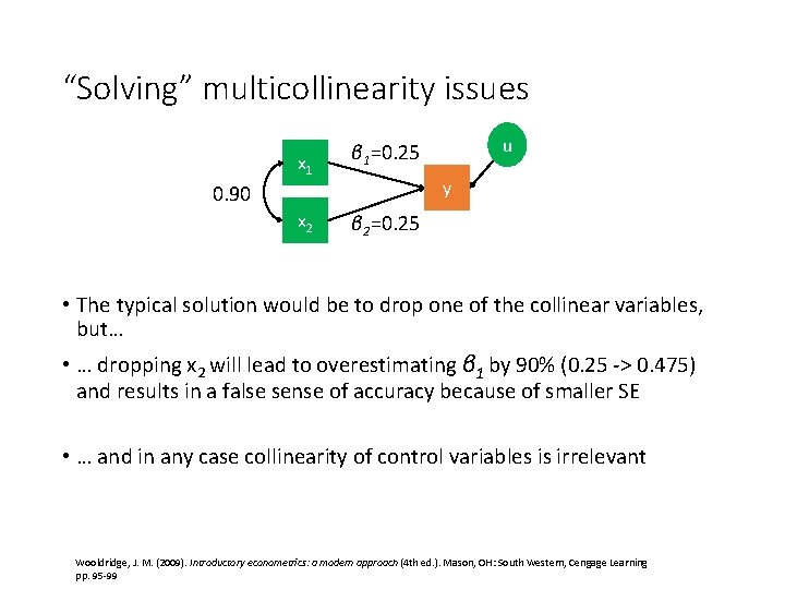
“Solving” multicollinearity issues x 1 β 1=0. 25 x 2 β 2=0. 25 u y 0. 90 • The typical solution would be to drop one of the collinear variables, but… • … dropping x 2 will lead to overestimating β 1 by 90% (0. 25 -> 0. 475) and results in a false sense of accuracy because of smaller SE • … and in any case collinearity of control variables is irrelevant Wooldridge, J. M. (2009). Introductory econometrics: a modern approach (4 th ed. ). Mason, OH: South Western, Cengage Learning pp. 95 -99

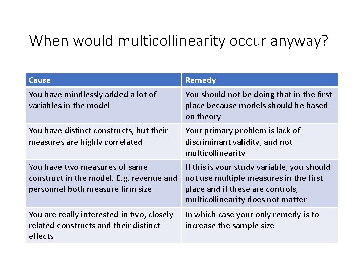
When would multicollinearity occur anyway? Cause Remedy You have mindlessly added a lot of variables in the model You should not be doing that in the first place because models should be based on theory You have distinct constructs, but their measures are highly correlated Your primary problem is lack of discriminant validity, and not multicollinearity You have two measures of same If this is your study variable, you should construct in the model. E. g. revenue and not use multiple measures in the first personnel both measure firm size place and if these are controls, multicollinearity does not matter You are really interested in two, closely related constructs and their distinct effects In which case your only remedy is to increase the sample size

Let’s rethink this Hekman, D. R. , Aquino, K. , Owens, B. P. , Mitchell, T. R. , Schilpzand, P. , & Leavitt, K. (2010). An Examination of Whether and How Racial and Gender Biases Influence Customer Satisfaction. Academy of Management Journal, 53(2), 238– 264. doi: 10. 5465/AMJ. 2010. 49388763 p. 258

What does this mean? Deephouse, D. L. (1999). To be different, or to be the same? It’s a question (and theory) of strategic balance. Strategic Management Journal, 20(2), 147– 166. https: //doi. org/10. 1002/(SICI)1097 -0266(199902)20: 2<147: : AID-SMJ 11>3. 0. CO; 2 -Q , p. 159

Mediation

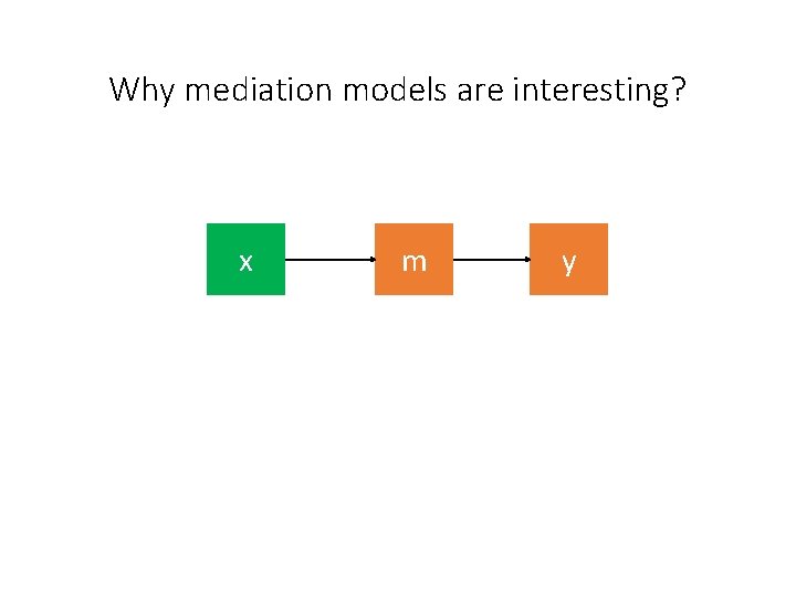
Why mediation models are interesting? x m y

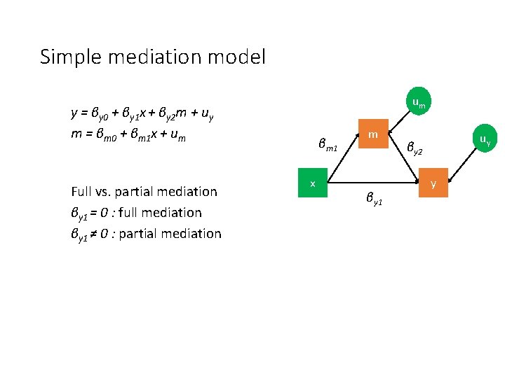
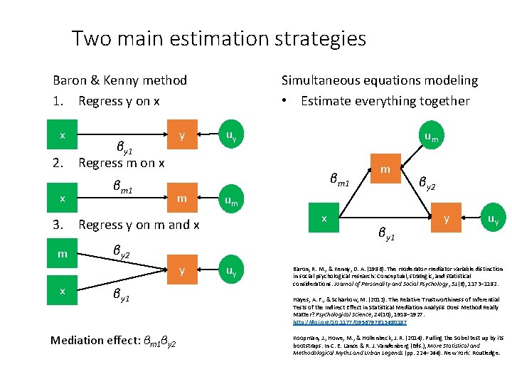
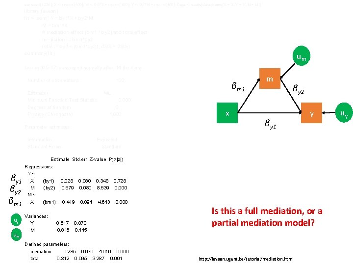
Simple mediation model um y = βy 0 + βy 1 x + βy 2 m + uy m = βm 0 + βm 1 x + um Full vs. partial mediation βy 1 = 0 : full mediation βy 1 ≠ 0 : partial mediation βm 1 x m βy 1 uy βy 2 y

Two main estimation strategies Baron & Kenny method 1. Regress y on x x 2. x βy 1 Regress m on x βm 1 y Simultaneous equations modeling • Estimate everything together uy βm 1 m x βy 2 y x βy 1 Mediation effect: βm 1βy 2 m um 3. Regress y on m and x m um uy βy 1 βy 2 y uy Baron, R. M. , & Kenny, D. A. (1986). The moderator-mediator variable distinction in social psychological research: Conceptual, strategic, and statistical considerations. Journal of Personality and Social Psychology, 51(6), 1173– 1182. Hayes, A. F. , & Scharkow, M. (2013). The Relative Trustworthiness of Inferential Tests of the Indirect Effect in Statistical Mediation Analysis Does Method Really Matter? Psychological Science, 24(10), 1918– 1927. http: //doi. org/10. 1177/0956797613480187 Koopman, J. , Howe, M. , & Hollenbeck, J. R. (2014). Pulling the Sobel test up by its bootstraps. In C. E. Lance & R. J. Vandenberg (Eds. ), More Statistical and Methodological Myths and Urban Legends (pp. 224– 244). New York: Routledge.

Baron and Kenny (1986) approach to mediation

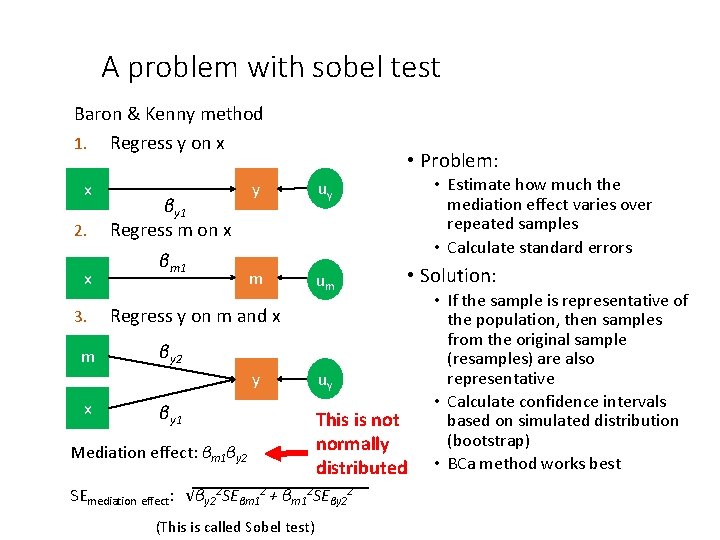
A problem with sobel test Baron & Kenny method 1. Regress y on x x 2. x 3. m βy 1 Regress m on x βm 1 y uy m um • Estimate how much the mediation effect varies over repeated samples • Calculate standard errors • Solution: Regress y on m and x βy 2 y x • Problem: βy 1 Mediation effect: βm 1βy 2 uy This is not normally distributed SEmediation effect: √βy 22 SEβm 12 + βm 12 SEβy 22 (This is called Sobel test) • If the sample is representative of the population, then samples from the original sample (resamples) are also representative • Calculate confidence intervals based on simulated distribution (bootstrap) • BCa method works best

Bootstrapping

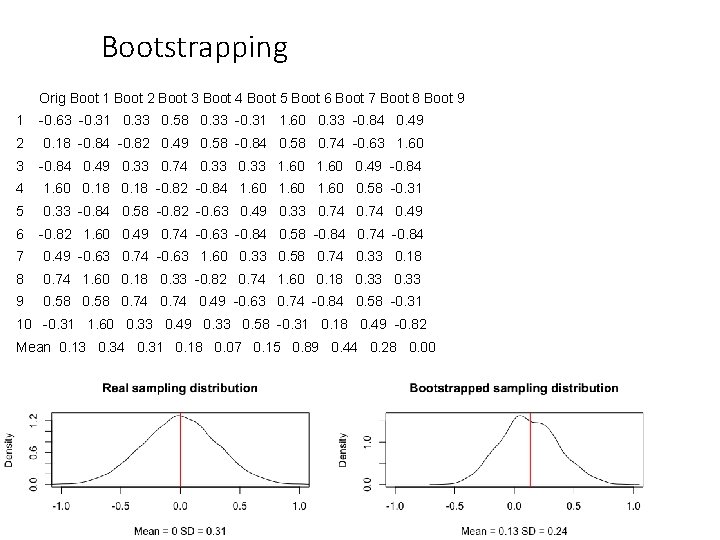
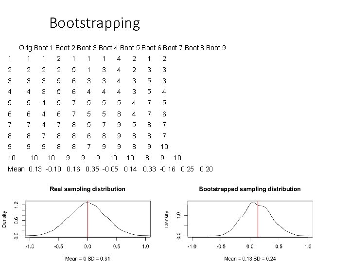
Bootstrapping Orig Boot 1 Boot 2 Boot 3 Boot 4 Boot 5 Boot 6 Boot 7 Boot 8 Boot 9 1 -0. 63 -0. 31 0. 33 0. 58 0. 33 -0. 31 1. 60 0. 33 -0. 84 0. 49 2 0. 18 -0. 84 -0. 82 0. 49 0. 58 -0. 84 0. 58 0. 74 -0. 63 1. 60 3 -0. 84 0. 49 0. 33 0. 74 0. 33 1. 60 0. 49 -0. 84 4 1. 60 0. 18 -0. 82 -0. 84 1. 60 0. 58 -0. 31 5 0. 33 -0. 84 0. 58 -0. 82 -0. 63 0. 49 0. 33 0. 74 0. 49 6 -0. 82 1. 60 0. 49 0. 74 -0. 63 -0. 84 0. 58 -0. 84 0. 74 -0. 84 7 0. 49 -0. 63 0. 74 -0. 63 1. 60 0. 33 0. 58 0. 74 0. 33 0. 18 8 0. 74 1. 60 0. 18 0. 33 -0. 82 0. 74 1. 60 0. 18 0. 33 9 0. 58 0. 74 0. 49 -0. 63 0. 74 -0. 84 0. 58 -0. 31 10 -0. 31 1. 60 0. 33 0. 49 0. 33 0. 58 -0. 31 0. 18 0. 49 -0. 82 Mean 0. 13 0. 34 0. 31 0. 18 0. 07 0. 15 0. 89 0. 44 0. 28 0. 00

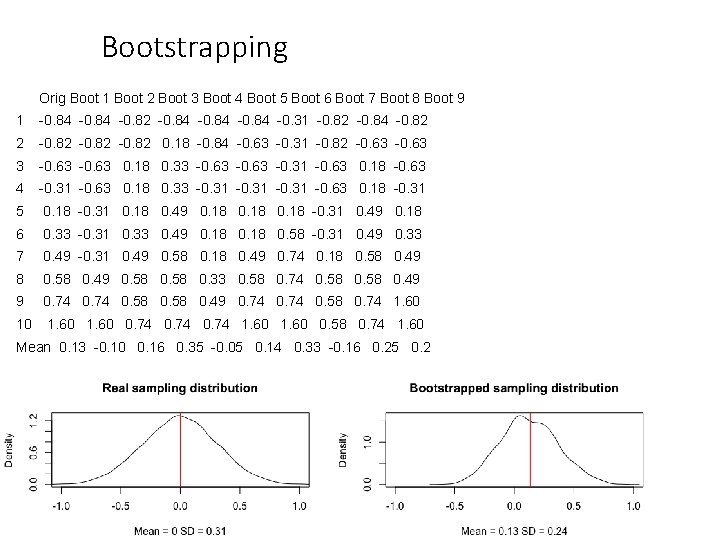
Bootstrapping Orig Boot 1 Boot 2 Boot 3 Boot 4 Boot 5 Boot 6 Boot 7 Boot 8 Boot 9 1 -0. 84 -0. 82 -0. 84 -0. 31 -0. 82 -0. 84 -0. 82 2 -0. 82 0. 18 -0. 84 -0. 63 -0. 31 -0. 82 -0. 63 3 -0. 63 0. 18 0. 33 -0. 63 -0. 31 -0. 63 0. 18 -0. 63 4 -0. 31 -0. 63 0. 18 0. 33 -0. 31 -0. 63 0. 18 -0. 31 5 0. 18 -0. 31 0. 18 0. 49 0. 18 -0. 31 0. 49 0. 18 6 0. 33 -0. 31 0. 33 0. 49 0. 18 0. 58 -0. 31 0. 49 0. 33 7 0. 49 -0. 31 0. 49 0. 58 0. 18 0. 49 0. 74 0. 18 0. 58 0. 49 0. 58 0. 33 0. 58 0. 74 0. 58 0. 49 9 0. 74 0. 58 0. 49 0. 74 0. 58 0. 74 1. 60 10 1. 60 0. 74 1. 60 0. 58 0. 74 1. 60 Mean 0. 13 -0. 10 0. 16 0. 35 -0. 05 0. 14 0. 33 -0. 16 0. 25 0. 2

Bootstrapping Orig Boot 1 Boot 2 Boot 3 Boot 4 Boot 5 Boot 6 Boot 7 Boot 8 Boot 9 1 1 1 2 1 1 1 4 2 1 2 2 2 5 1 3 4 2 3 3 3 5 6 3 3 4 3 5 3 4 4 3 5 6 4 4 4 3 5 4 5 7 5 5 5 4 7 5 6 6 4 6 7 5 5 8 4 7 6 7 7 4 7 8 5 7 9 5 8 7 8 8 6 8 9 8 8 7 9 9 8 9 10 10 10 9 9 9 10 10 Mean 0. 13 -0. 10 0. 16 0. 35 -0. 05 0. 14 0. 33 -0. 16 0. 25 0. 20

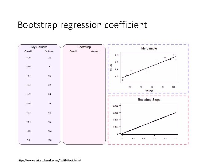
Bootstrap regression coefficient https: //www. stat. auckland. ac. nz/~wild/Boot. Anim/

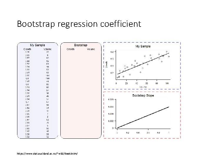
Bootstrap regression coefficient https: //www. stat. auckland. ac. nz/~wild/Boot. Anim/

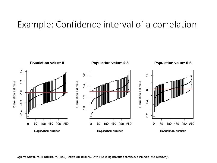
Example: Confidence interval of a correlation Aguirre-Urreta, M. , & Rönkkö, M. (2018). Statistical inference with PLSc using bootstrap confidence intervals. MIS Quarterly.

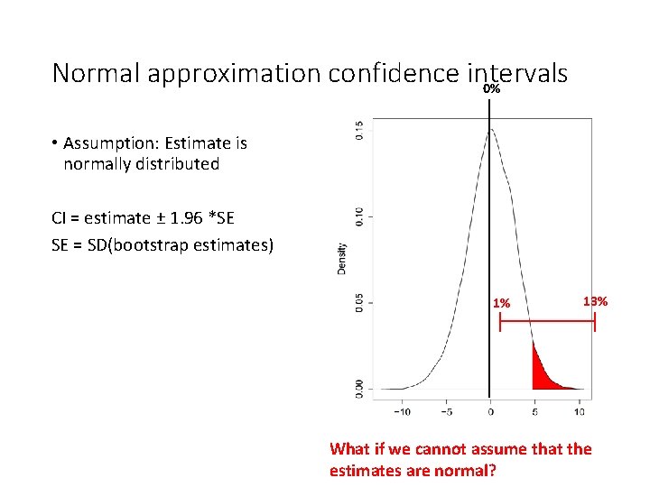
Normal approximation confidence intervals 0% • Assumption: Estimate is normally distributed CI = estimate ± 1. 96 *SE SE = SD(bootstrap estimates) 1% 13% What if we cannot assume that the estimates are normal?

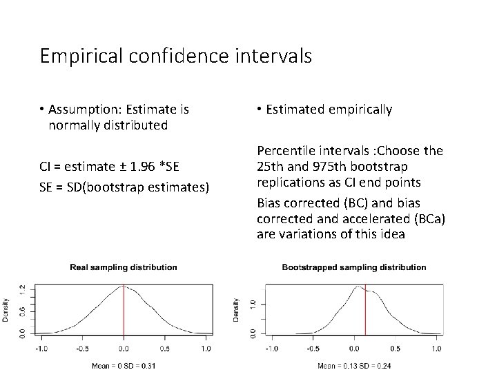
Empirical confidence intervals • Assumption: Estimate is normally distributed CI = estimate ± 1. 96 *SE SE = SD(bootstrap estimates) • Estimated empirically Percentile intervals : Choose the 25 th and 975 th bootstrap replications as CI end points Bias corrected (BC) and bias corrected and accelerated (BCa) are variations of this idea

When does it work? Koopman et al (2014, p. 229): 1. Bootstrapping has been advocated as being particularly useful in small samples (e. g. , Shrout & Bolger, 2002). 2. Bootstrapping necessarily assumes that a sample is representative of the population (Mooney & Duval, 1993). 3. Sampling error is particularly troublesome in small samples, rendering an assumption that a sample is representative of the population in this context tenuous at best (Schmidt, Hunter, & Pearlman, 1981). ⇒ Bootstrapping requires a large sample size Koopman, J. , Howe, M. , & Hollenbeck, J. R. (2014). Pulling the Sobel test up by its bootstraps. In C. E. Lance & R. J. Vandenberg (Eds. ), More statistical and methodological myths and urban legends (pp. 224– 244). New York: Routledge. Koopman, J. , Howe, M. , Hollenbeck, J. R. , & Sin, H. -P. (2015). Small sample mediation testing: Misplaced confidence in bootstrapped confidence intervals. Journal of Applied Psychology, 100(1), 194– 202.

Simultaneous equations approach to mediation

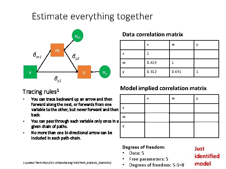
Estimate everything together Data correlation matrix um βm 1 x m βy 1 x βy 2 y uy Tracing rules 1 • • • x 1 m 0. 419 1 y 0. 312 0. 691 y 1 Model implied correlation matrix You can trace backward up an arrow and then forward along the next, or forwards from one x variable to the other, but never forward and then back. m You can pass through each variable only once in a y given chain of paths. No more than one bi-directional arrow can be included in each path-chain. 1 quoted from http: //en. wikipedia. org/wiki/Path_analysis_(statistics) m x m y 1 βm 12 + var(um) βm 1 βy 2 + βy 1 βy 2 + βm 1 βy 1 Degrees of freedom: • Data: 5 • Free parameters: 5 • Degrees of freedom: 5 -5=0 βy 12 + βy 22 + 2βy 1βm 2βy 2 + var(uy) Just identified model

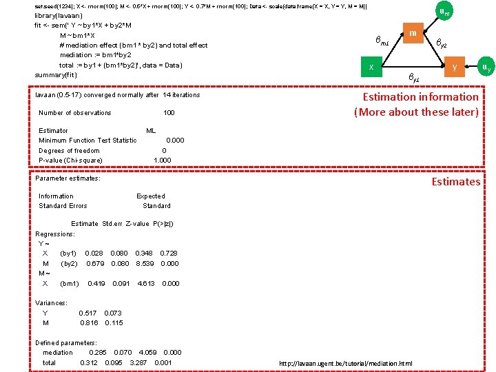
set. seed(1234); X <- rnorm(100); M <- 0. 5*X + rnorm(100); Y <- 0. 7*M + rnorm(100); Data <- scale(data. frame(X = X, Y = Y, M = M)) library(lavaan) fit <- sem(' Y ~ by 1*X + by 2*M M ~ bm 1*X # mediation effect (bm 1 * by 2) and total effect mediation : = bm 1*by 2 total : = by 1 + (bm 1*by 2)', data = Data) summary(fit) βm 1 x 100 Estimator Minimum Function Test Statistic Degrees of freedom P-value (Chi-square) m βy 1 y ML 0. 000 0 1. 000 Estimates Parameter estimates: Information Standard Errors βy 2 Estimation information (More about these later) lavaan (0. 5 -17) converged normally after 14 iterations Number of observations um Expected Standard Estimate Std. err Z-value P(>|z|) Regressions: Y~ X (by 1) 0. 028 0. 080 0. 348 0. 728 M (by 2) 0. 679 0. 080 8. 539 0. 000 M~ X (bm 1) 0. 419 0. 091 4. 613 0. 000 Variances: Y M 0. 517 0. 073 0. 816 0. 115 Defined parameters: mediation 0. 285 0. 070 4. 059 0. 000 total 0. 312 0. 095 3. 287 0. 001 28. 2. 2021 45 http: //lavaan. ugent. be/tutorial/mediation. html uy

set. seed(1234); X <- rnorm(100); M <- 0. 5*X + rnorm(100); Y <- 0. 7*M + rnorm(100); Data <- scale(data. frame(X = X, Y = Y, M = M)) library(lavaan) fit <- sem(' Y ~ by 1*X + by 2*M M ~ bm 1*X # mediation effect (bm 1 * by 2) and total effect mediation : = bm 1*by 2 total : = by 1 + (bm 1*by 2)', data = Data) summary(fit) um lavaan (0. 5 -17) converged normally after 14 iterations Number of observations 100 Estimator Minimum Function Test Statistic Degrees of freedom P-value (Chi-square) βy 1 βy 2 βm 1 0 1. 000 uy um x βy 1 y Expected Standard Estimate Std. err Z-value P(>|z|) Regressions: Y~ X (by 1) 0. 028 0. 080 0. 348 0. 728 M (by 2) 0. 679 0. 080 8. 539 0. 000 M~ X (bm 1) 0. 419 0. 091 4. 613 0. 000 Variances: Y M βy 2 0. 000 Parameter estimates: Information Standard Errors βm 1 ML m 0. 517 0. 073 0. 816 0. 115 Defined parameters: mediation 0. 285 0. 070 4. 059 0. 000 total 0. 312 0. 095 3. 287 0. 001 Is this a full mediation, or a partial mediation model? http: //lavaan. ugent. be/tutorial/mediation. html uy

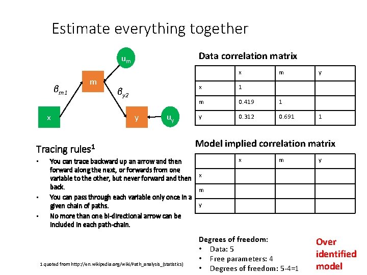
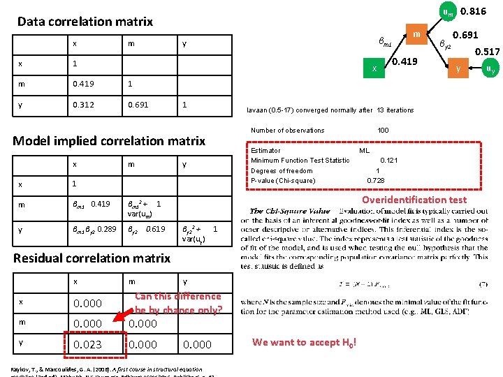
Estimate everything together Data correlation matrix um βm 1 m x x βy 2 y uy Tracing rules 1 • • • x 1 m 0. 419 1 y 0. 312 0. 691 y 1 Model implied correlation matrix You can trace backward up an arrow and then forward along the next, or forwards from one x variable to the other, but never forward and then back. m You can pass through each variable only once in a y given chain of paths. No more than one bi-directional arrow can be included in each path-chain. 1 quoted from http: //en. wikipedia. org/wiki/Path_analysis_(statistics) m x m y 1 βm 12 + var(um) βm 1 βy 2 Degrees of freedom: • Data: 5 • Free parameters: 4 • Degrees of freedom: 5 -4=1 βy 22 + var(uy) Over identified model

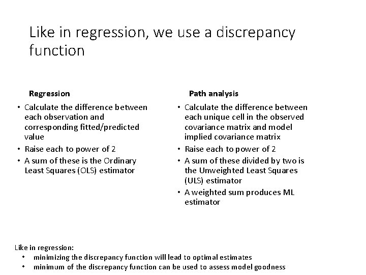
Like in regression, we use a discrepancy function Regression • Calculate the difference between each observation and corresponding fitted/predicted value • Raise each to power of 2 • A sum of these is the Ordinary Least Squares (OLS) estimator • • Path analysis Calculate the difference between each unique cell in the observed covariance matrix and model implied covariance matrix Raise each to power of 2 A sum of these divided by two is the Unweighted Least Squares (ULS) estimator A weighted sum produces ML estimator Like in regression: • minimizing the discrepancy function will lead to optimal estimates • minimum of the discrepancy function can be used to assess model goodness

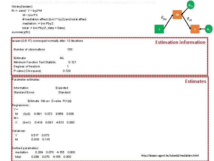
set. seed(1234); X <- rnorm(100); M <- 0. 5*X + rnorm(100); Y <- 0. 7*M + rnorm(100); Data <- scale(data. frame(X = X, Y = Y, M = M)) library(lavaan) fit <- sem(' Y ~ by 2*M M ~ bm 1*X # mediation effect (bm 1 * by 2) and total effect mediation : = bm 1*by 2 total : = bm 1*by 2', data = Data) summary(fit) βm 1 x βy 2 y 100 Estimator Minimum Function Test Statistic Degrees of freedom P-value (Chi-square) ML 0. 121 1 0. 728 Parameter estimates: Information Standard Errors m Estimation information lavaan (0. 5 -17) converged normally after 13 iterations Number of observations um Estimates Expected Standard Estimate Std. err Z-value P(>|z|) Regressions: Y~ M (by 2) 0. 691 0. 072 9. 559 0. 000 M~ X (bm 1) 0. 419 0. 091 4. 613 0. 000 Variances: Y M 0. 517 0. 073 0. 816 0. 115 Defined parameters: mediation 0. 289 0. 070 4. 155 0. 000 total 0. 289 0. 070 4. 155 0. 000 28. 2. 2021 49 http: //lavaan. ugent. be/tutorial/mediation. html uy

um 0. 816 Data correlation matrix x m x 1 m 0. 419 1 y 0. 312 0. 691 m 1 1 m βm 1 0. 419 βm 12 + 1 var(um) y βm 1 βy 2 0. 289 βy 2 0. 619 Number of observations Estimator Minimum Function Test Statistic Degrees of freedom P-value (Chi-square) βy 22 + var(uy) 1 y Can this difference be by chance only? x 0. 000 m 0. 000 y 0. 023 0. 000 0. 691 0. 517 y 100 ML 0. 121 1 0. 728 Overidentification test Residual correlation matrix m βy 2 lavaan (0. 5 -17) converged normally after 13 iterations y x x 0. 419 x Model implied correlation matrix x m βm 1 y 0. 000 Raykov, T. , & Marcoulides, G. A. (2006). A first course in structural equation We want to accept H 0! uy

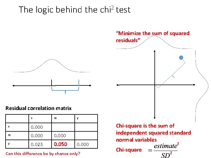
The logic behind the chi 2 test “Minimize the sum of squared residuals” Residual correlation matrix x m x 0. 000 m 0. 000 y 0. 023 0. 000 0. 050 y 0. 000 Can this difference be by chance only? Chi-square is the sum of independent squared standard normal variables 2 Chi-square 2