Linear filters and edges Linear Filters l General

Linear filters and edges

Linear Filters l General process: l l Form new image whose pixels are a weighted sum of original pixel values, using the same set of weights at each point. l l l Properties l l Example: smoothing by averaging Output is a linear function of the input l Output is a shift-invariant function of the input (i. e. shift the input image two pixels to the left, the output is shifted two pixels to the left) form the average of pixels in a neighborhood Example: smoothing with a Gaussian l form a weighted average of pixels in a neighborhood Example: finding a derivative l form a weighted average of pixels in a neighborhood

Convolution l l l Represent these weights as an image, H H is usually called the kernel Operation is called convolution l it’s associative l Result is: l Notice weird order of indices l l all examples can be put in this form it’s a result of the derivation expressing any shift-invariant linear operator as a convolution.

Convolution f(. ) f(. ) c 11 c 12 c 13 c 21 c 22 c 23 c 31 c 32 c 33 o (i, j) = c 11 f(i-1, j-1) + c 12 f(i-1, j) + c 13 f(i-1, j+1) + c 21 f(i, j-1) + c 22 f(i, j) c 31 f(i+1, j-1) + c 32 f(i+1, j) + c 33 f(i+1, j+1) + c 23 f(i, j+1) +

Example: Smoothing by Averaging

Smoothing with a Gaussian l Smoothing with an average actually doesn’t compare at all well with a de-focused lens l Most obvious difference is that a single point of light viewed in a defocused lens looks like a fuzzy blob; but the averaging process would give a little square. l A Gaussian gives a good model of a fuzzy blob

An Isotropic Gaussian l The picture shows a smoothing kernel proportional to (which is a reasonable model of a circularly symmetric fuzzy blob)

Smoothing with a Gaussian

Differentiation and convolution We could approximate this as l Recall l l Now this is linear and shift invariant, so must be the result of a convolution. (which is obviously a convolution; it’s not a very good way to do things, as we shall see)

Finite differences

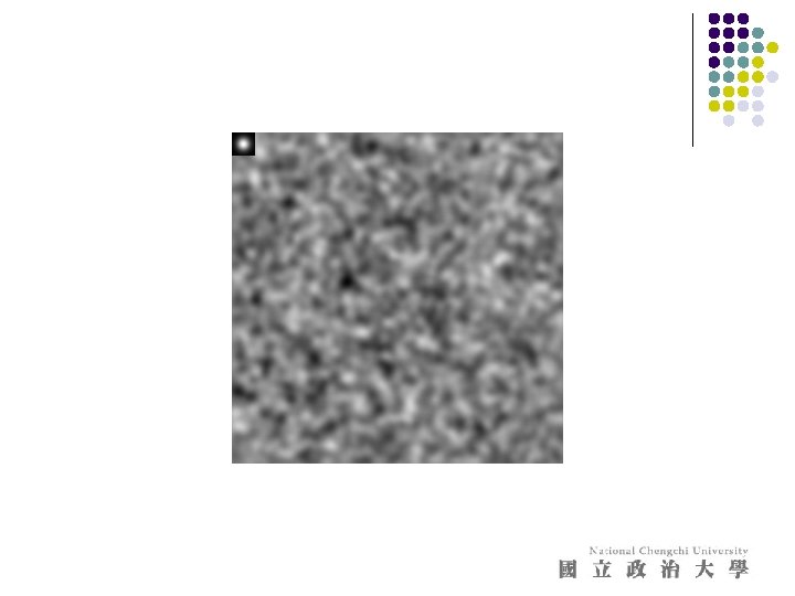
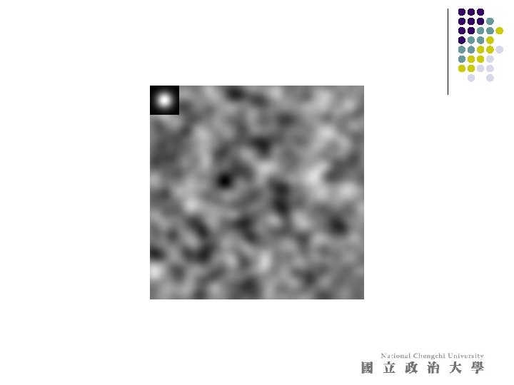
Noise l Simplest noise model l l independent stationary additive Gaussian noise the noise value at each pixel is given by an independent draw from the same normal probability distribution l Issues l l this model allows noise values that could be greater than maximum camera output or less than zero for small standard deviations, this isn’t too much of a problem - it’s a fairly good model independence may not be justified (e. g. damage to lens) may not be stationary (e. g. thermal gradients in the ccd)

sigma=1

sigma=16

Finite differences and noise l Finite difference filters respond strongly to noise l l obvious reason: image noise results in pixels that look very different from their neighbors Generally, the larger the noise the stronger the response l What is to be done? l l l intuitively, most pixels in images look quite a lot like their neighbors this is true even at an edge; along the edge they’re similar, across the edge they’re not suggests that smoothing the image should help, by forcing pixels different to their neighbors (=noise pixels? ) to look more like neighbors

Finite differences responding to noise Increasing noise -> (this is zero mean additive gaussian noise)

The response of a linear filter to noise l l Do only stationary independent additive Gaussian noise with zero mean (non-zero mean is easily dealt with) l Variance: l Mean: l l l output is a weighted sum of inputs so we want mean of a weighted sum of zero mean normal random variables must be zero l recall l variance of a sum of random variables is sum of their variances l variance of constant times random variable is constant^2 times variance then if s is noise variance and kernel is K, variance of response is

Filter responses are correlated l l over scales similar to the scale of the filter Filtered noise is sometimes useful l looks like some natural textures, can be used to simulate fire, etc.

Smoothing reduces noise l Generally expect pixels to “be like” their neighbors l l l surfaces turn slowly relatively few reflectance changes Generally expect noise processes to be independent from pixel to pixel l l Implies that smoothing suppresses noise, for appropriate noise models Scale l l the parameter in the symmetric Gaussian as this parameter goes up, more pixels are involved in the average and the image gets more blurred and noise is more effectively suppressed

The effects of smoothing Each row shows smoothing with gaussians of different width; each column shows different realizations of an image of gaussian noise.

Some other useful filtering techniques l l Median filter Anisotropic diffusion

Median filters : principle non-linear filter method : n 1. rank-order neighborhood intensities n 2. take middle value no new gray levels emerge. . .

Median filters : odd-man-out advantage of this type of filter is its “odd-man-out” effect e. g. 1, 1, 1, 7, 1, 1 ? , 1, 1, 1, ?

Median filters : example filters have width 5 :

Median filters : analysis median completely discards the spike, linear filter always responds to all aspects median filter preserves discontinuities, linear filter produces rounding-off effects DON’T become all too optimistic

Median filter : images 3 x 3 median filter : sharpens edges, destroys edge cusps and protrusions

Median filters : Gauss revisited Comparison with Gaussian : e. g. upper lip smoother, eye better preserved

Example of median 10 times 3 X 3 median patchy effect important details lost (e. g. ear-ring)

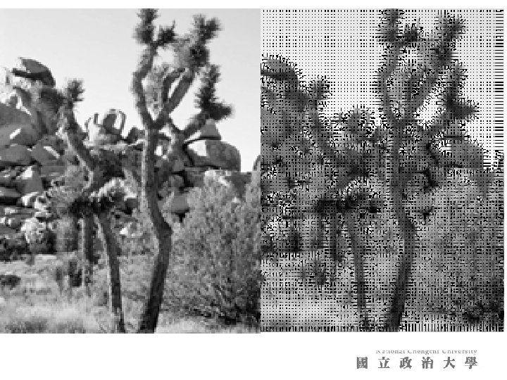
Gradients and edges l Points of sharp change in an image are interesting: l l l change in reflectance change in object change in illumination noise Sometimes called edge points l General strategy l determine image gradient l now mark points where gradient magnitude is particularly large wrt neighbors (ideally, curves of such points).

There are three major issues: 1) The gradient magnitude at different scales is different; which should we choose? 2) The gradient magnitude is large along thick trail; how do we identify the significant points? 3) How do we link the relevant points up into curves?

Smoothing and Differentiation l Issue: noise l l l smooth before differentiation two convolutions to smooth, then differentiate? actually, no - we can use a derivative of Gaussian filter l because differentiation is convolution, and convolution is associative

1 pixel 3 pixels 7 pixels The scale of the smoothing filter affects derivative estimates, and also the semantics of the edges recovered.

We wish to mark points along the curve where the magnitude is biggest. We can do this by looking for a maximum along a slice normal to the curve (non-maximum suppression). These points should form a curve. There are then two algorithmic issues: at which point is the maximum, and where is the next one?

Non-maximum suppression At q, we have a maximum if the value is larger than those at both p and at r. Interpolate to get these values.

Predicting the next edge point Assume the marked point is an edge point. Then we construct the tangent to the edge curve (which is normal to the gradient at that point) and use this to predict the next points (here either r or s).

Remaining issues l Check that maximum value of gradient value is sufficiently large l drop-outs? use hysteresis l use a high threshold to start edge curves and a low threshold to continue them.

Notice l l l Something nasty is happening at corners Scale affects contrast Edges are not bounding contours

fine scale high threshold

coarse scale, high threshold

coarse scale low threshold

Filters are templates l l Applying a filter at some point can be seen as taking a dot-product between the image and some vector Filtering the image is a set of dot products l Insight l l filters look like the effects they are intended to find filters find effects they look like

Normalized correlation l Think of filters of a dot product l l now measure the angle i. e normalized correlation output is filter output, divided by root sum of squares of values over which filter lies l Tricks: l l l ensure that filter has a zero response to a constant region (helps reduce response to irrelevant background) subtract image average when computing the normalizing constant (i. e. subtract the image mean in the neighborhood) absolute value deals with contrast reversal

Positive responses Zero mean image, -1: 1 scale Zero mean image, -max: max scale

Positive responses Zero mean image, -1: 1 scale Zero mean image, -max: max scale

Figure from “Computer Vision for Interactive Computer Graphics, ” W. Freeman et al, IEEE Computer Graphics and Applications, 1998 copyright 1998, IEEE

The Laplacian of Gaussian l l Another way to detect an extremal first derivative is to look for a zero second derivative Appropriate 2 D analogy is rotation invariant l the Laplacian l Bad idea to apply a Laplacian without smoothing l l l smooth with Gaussian, apply Laplacian this is the same as filtering with a Laplacian of Gaussian filter Now mark the zero points where there is a sufficiently large derivative, and enough contrast

sigma=4 contrast=1 LOG zero crossings sigma=2 contrast=4

We still have unfortunate behavior at corners

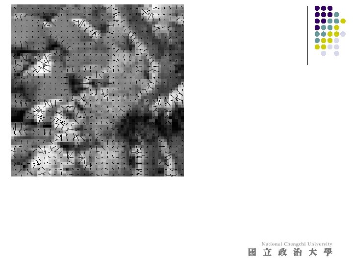
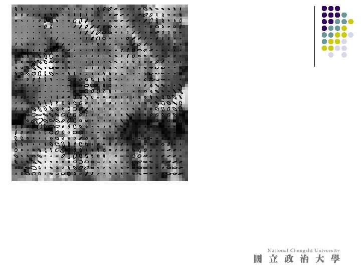
Orientation representations l The gradient magnitude is affected by illumination changes l l but it’s direction isn’t We can describe image patches by the swing of the gradient orientation l Important types: l l constant window l small gradient mags edge window l few large gradient mags in one direction flow window l many large gradient mags in one direction corner window l large gradient mags that swing

Representing Windows l Types l l constant l small eigenvalues Edge l one medium, one small Flow l one large, one small corner l two large eigenvalues