LINEAR CLASSIFIERS v The Problem Consider a two

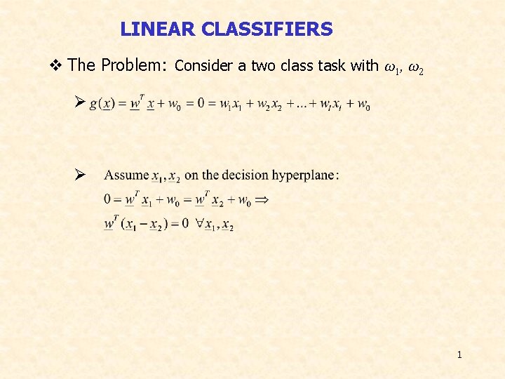
LINEAR CLASSIFIERS v The Problem: Consider a two class task with ω1, ω2 Ø Ø 1

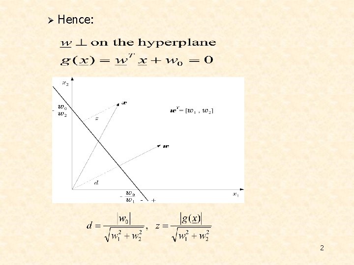
Ø Hence: 2

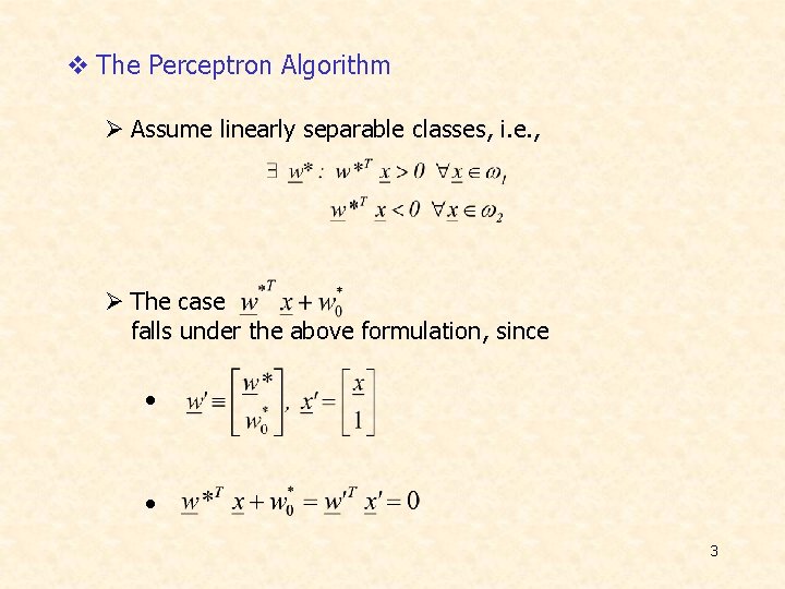
v The Perceptron Algorithm Ø Assume linearly separable classes, i. e. , Ø The case falls under the above formulation, since • • 3

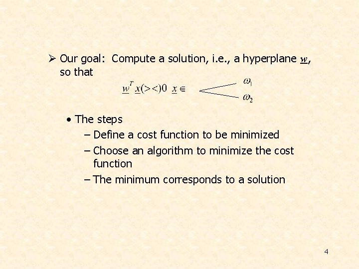
Ø Our goal: Compute a solution, i. e. , a hyperplane w, so that • The steps – Define a cost function to be minimized – Choose an algorithm to minimize the cost function – The minimum corresponds to a solution 4

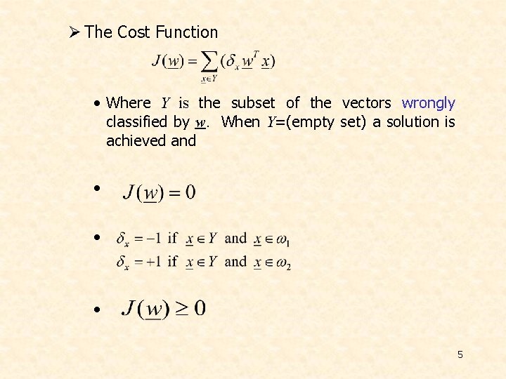
Ø The Cost Function • Where Y is the subset of the vectors wrongly classified by w. When Y=(empty set) a solution is achieved and • • • 5

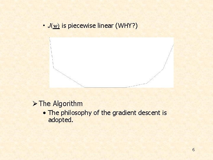
• J(w) is piecewise linear (WHY? ) Ø The Algorithm • The philosophy of the gradient descent is adopted. 6

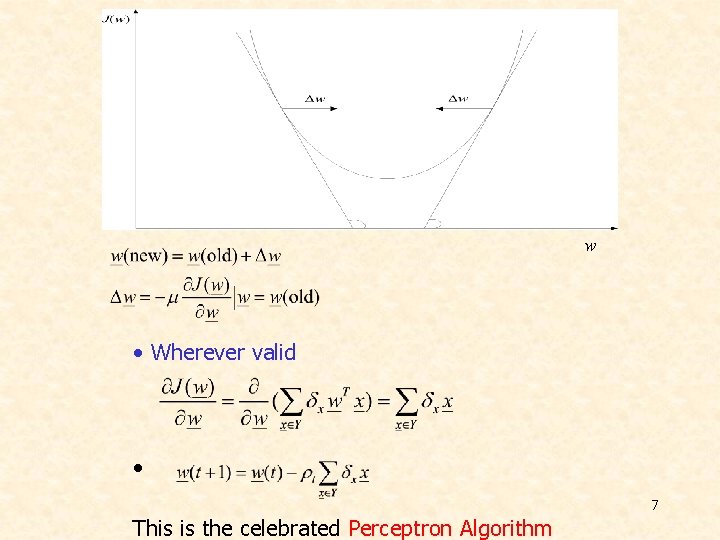
w • Wherever valid • 7 This is the celebrated Perceptron Algorithm

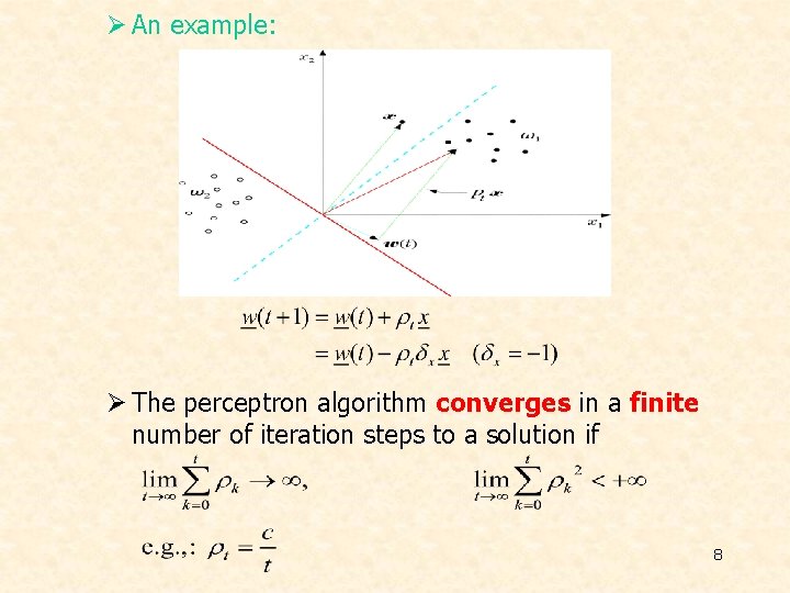
Ø An example: Ø The perceptron algorithm converges in a finite number of iteration steps to a solution if 8

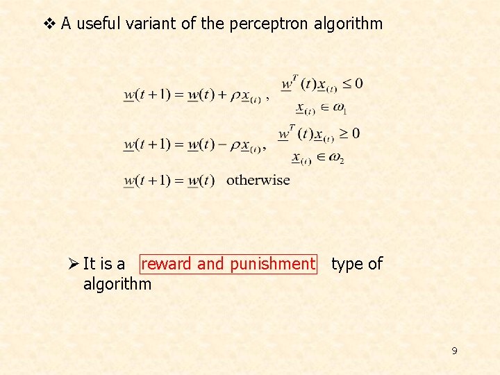
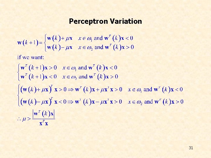
v A useful variant of the perceptron algorithm Ø It is a reward and punishment type of algorithm 9

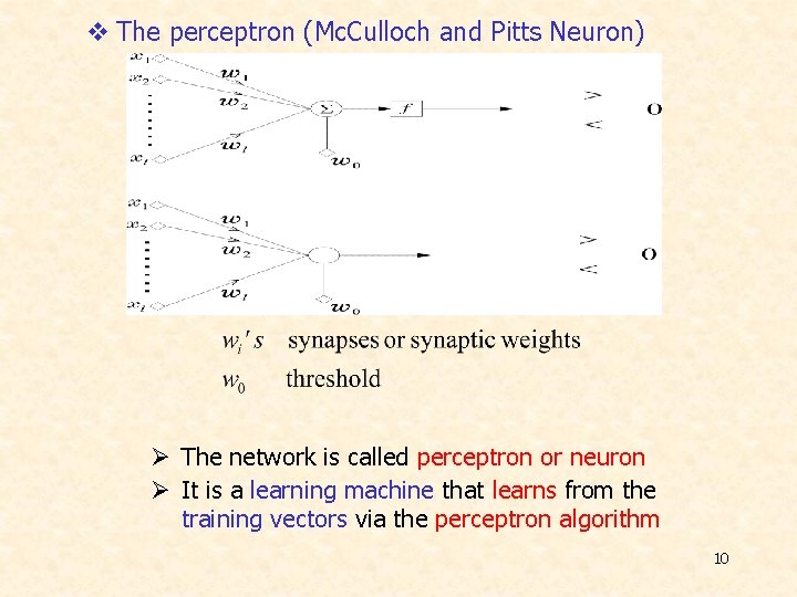
v The perceptron (Mc. Culloch and Pitts Neuron) Ø The network is called perceptron or neuron Ø It is a learning machine that learns from the training vectors via the perceptron algorithm 10

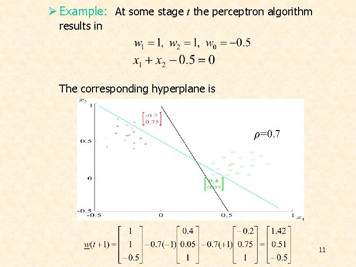
Ø Example: At some stage t the perceptron algorithm results in The corresponding hyperplane is ρ=0. 7 11

The Pocket Algorithm v Nonlinear Separable Ø Initialize the weight vector and history counter Ø Store best weight at our pocket! 12

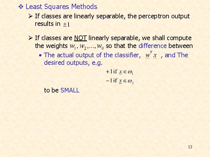
v Least Squares Methods Ø If classes are linearly separable, the perceptron output results in Ø If classes are NOT linearly separable, we shall compute the weights so that the difference between • The actual output of the classifier, , and The desired outputs, e. g. to be SMALL 13

Ø SMALL, in the mean square error sense, means to choose so that the cost function • • • 14

Ø Minimizing where Rx is the autocorrelation matrix and the crosscorrelation vector 15

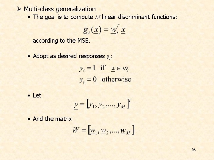
Ø Multi-class generalization • The goal is to compute M linear discriminant functions: according to the MSE. • Adopt as desired responses yi: • Let • And the matrix 16

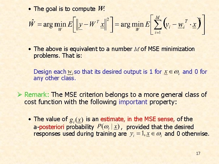
• The goal is to compute : • The above is equivalent to a number M of MSE minimization problems. That is: Design each so that its desired output is 1 for any other class. and 0 for Ø Remark: The MSE criterion belongs to a more general class of cost function with the following important property: • The value of is an estimate, in the MSE sense, of the a-posteriori probability , provided that the desired responses used during training are and 0 otherwise. 17

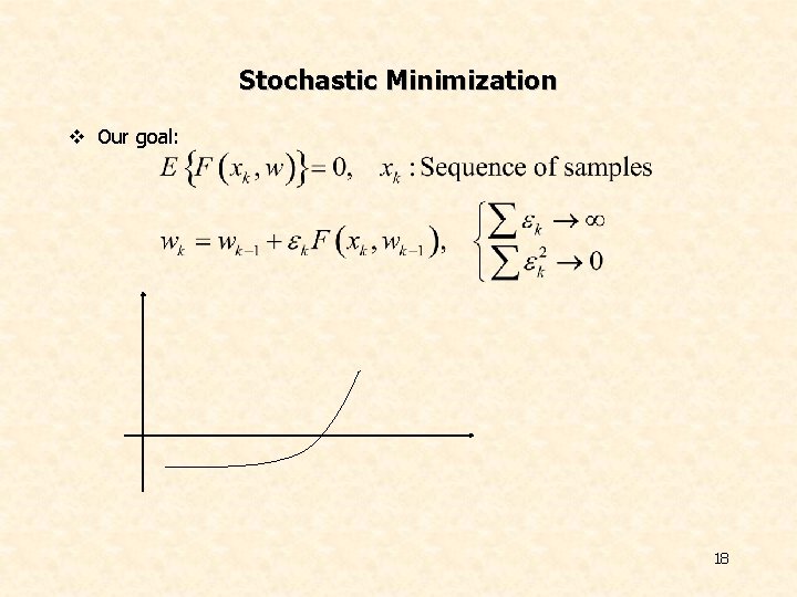
Stochastic Minimization v Our goal: 18

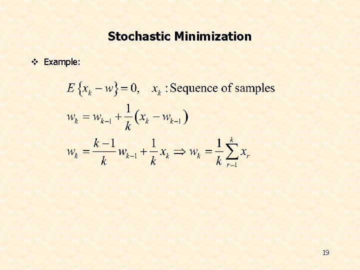
Stochastic Minimization v Example: 19

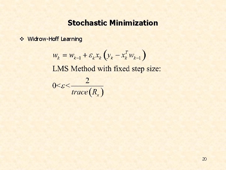
Stochastic Minimization v Widrow-Hoff Learning 20

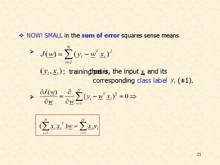
v NOW! SMALL in the sum of error squares sense means Ø is, the input xi and its : trainingthat pairs corresponding class label (± 1). Ø 21

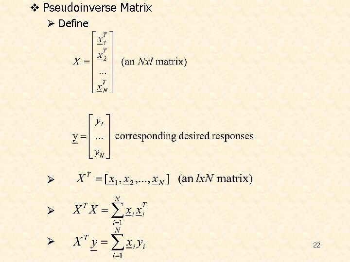
v Pseudoinverse Matrix Ø Define Ø Ø Ø 22

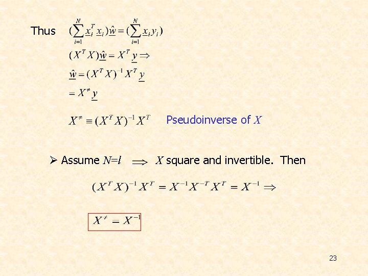
Thus Pseudoinverse of X Ø Assume N=l X square and invertible. Then 23

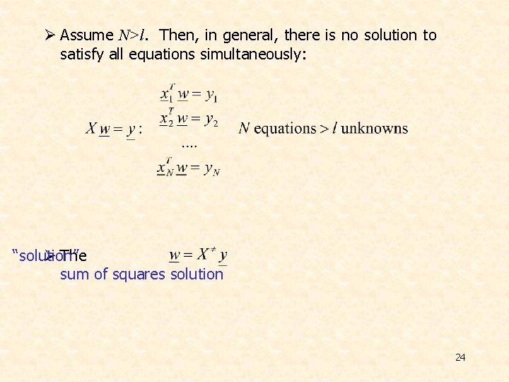
Ø Assume N>l. Then, in general, there is no solution to satisfy all equations simultaneously: “solution” Ø The sum of squares solution 24

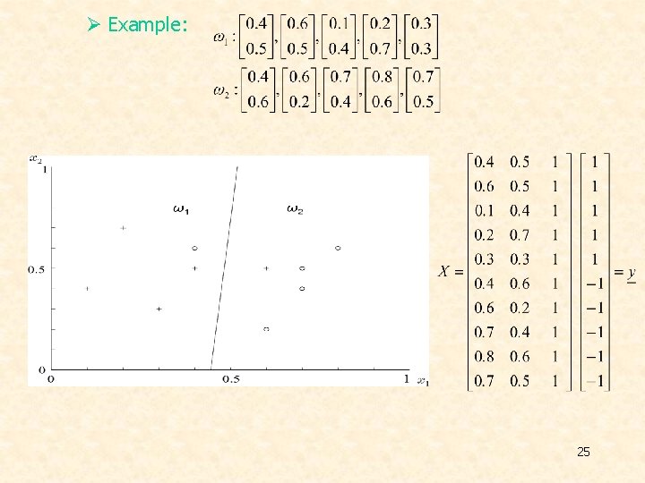
Ø Example: 25

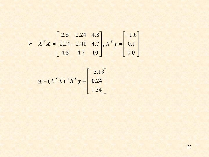
Ø 26

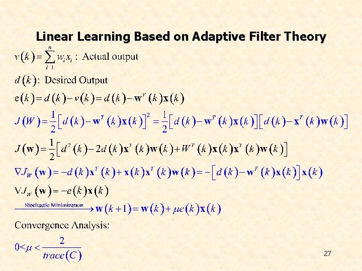
Linear Learning Based on Adaptive Filter Theory 27

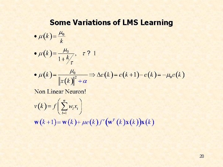
Some Variations of LMS Learning 28

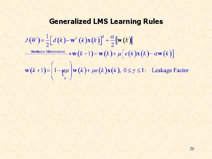
Generalized LMS Learning Rules 29

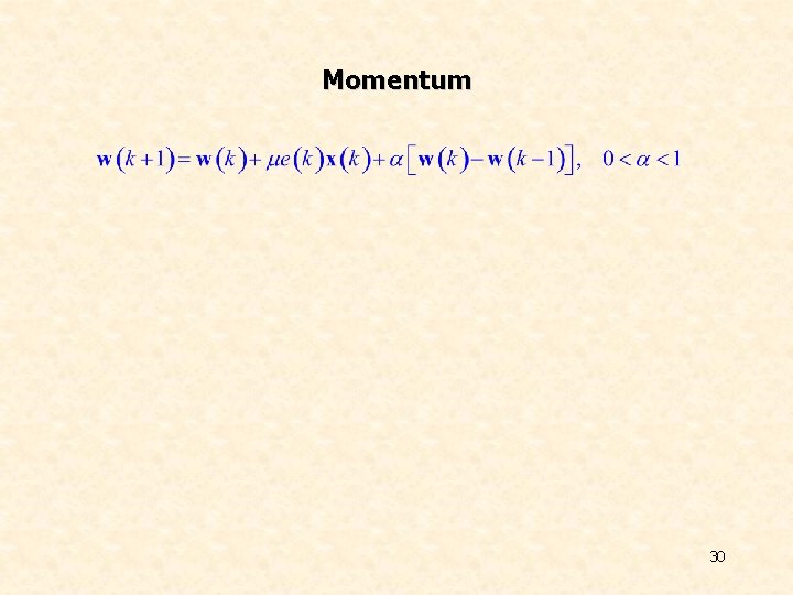
Momentum 30

Perceptron Variation 31

Marginal Methods v. Perceptron has many solutions! 32

Optimization Problem v. Non Constrained Problem v. Constrained Problem 33

Optimization Problem v. Constrained Problem 34

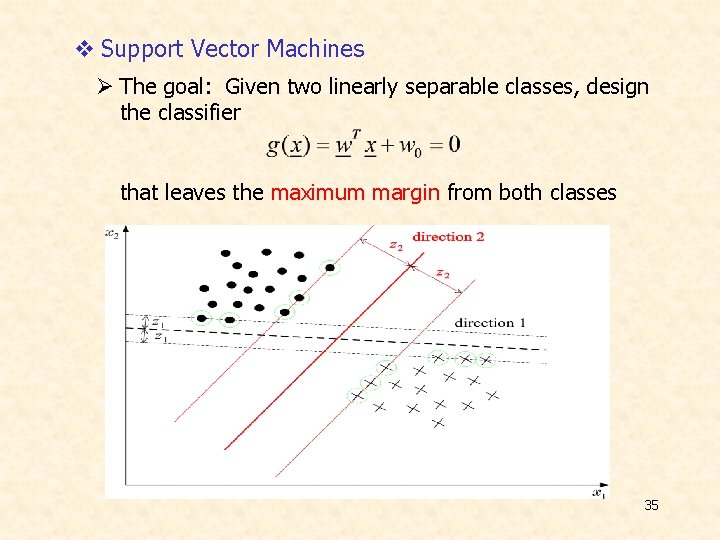
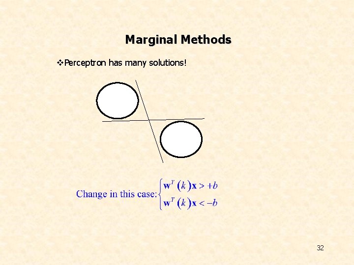
v Support Vector Machines Ø The goal: Given two linearly separable classes, design the classifier that leaves the maximum margin from both classes 35

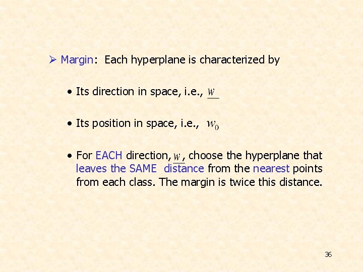
Ø Margin: Each hyperplane is characterized by • Its direction in space, i. e. , • Its position in space, i. e. , • For EACH direction, , choose the hyperplane that leaves the SAME distance from the nearest points from each class. The margin is twice this distance. 36

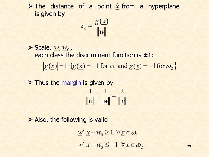
Ø The distance of a point is given by from a hyperplane Ø Scale, each class the discriminant function is ± 1: Ø Thus the margin is given by Ø Also, the following is valid 37

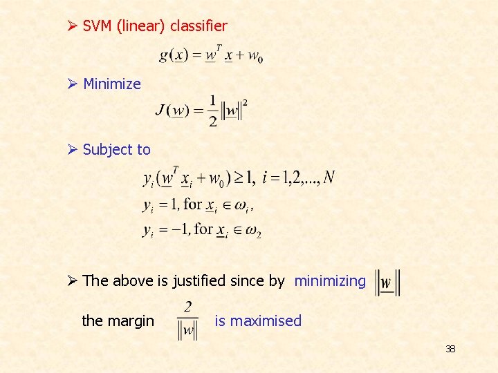
Ø SVM (linear) classifier Ø Minimize Ø Subject to Ø The above is justified since by minimizing the margin is maximised 38

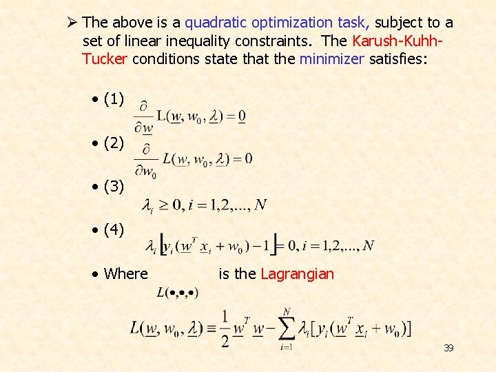
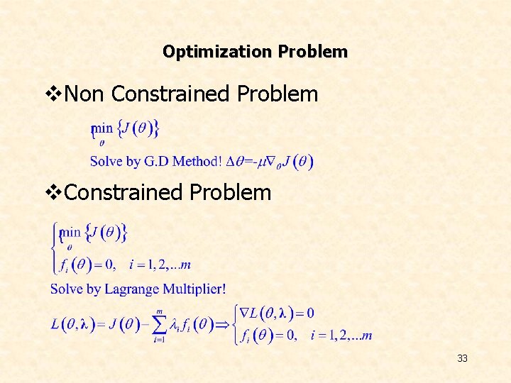
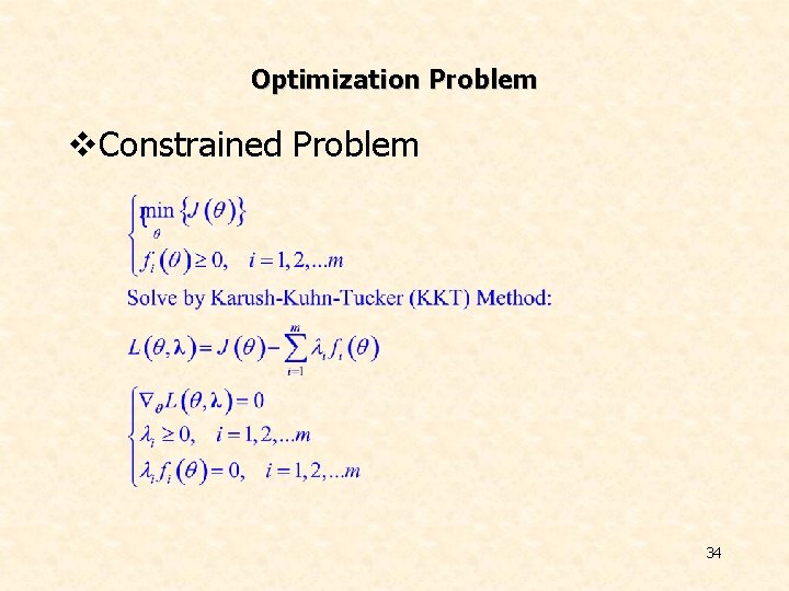
Ø The above is a quadratic optimization task, subject to a set of linear inequality constraints. The Karush-Kuhh. Tucker conditions state that the minimizer satisfies: • (1) • (2) • (3) • (4) • Where is the Lagrangian 39

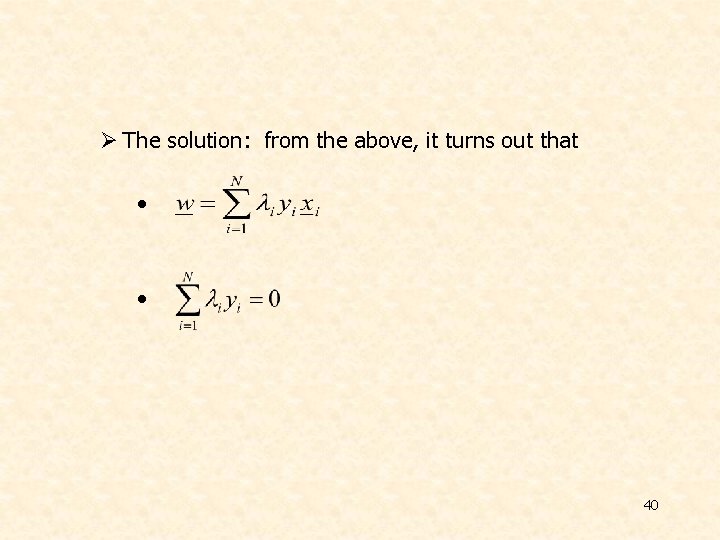
Ø The solution: from the above, it turns out that • • 40

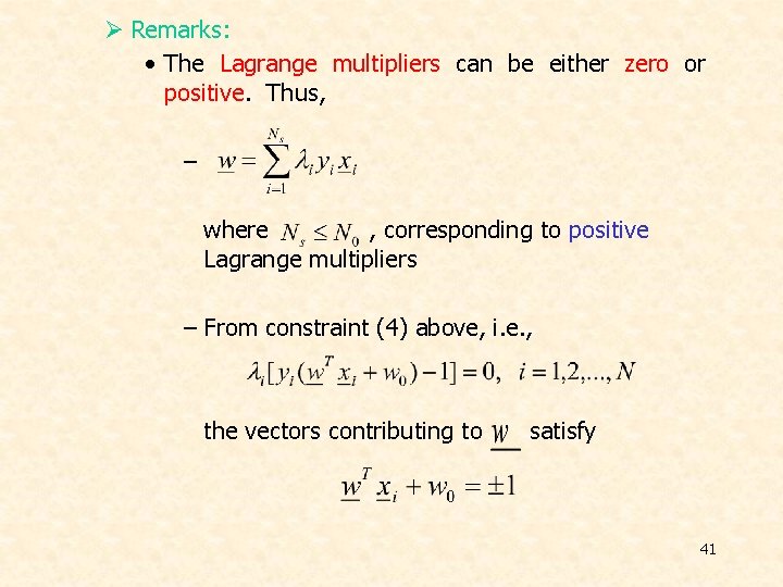
Ø Remarks: • The Lagrange multipliers can be either zero or positive. Thus, – where , corresponding to positive Lagrange multipliers – From constraint (4) above, i. e. , the vectors contributing to satisfy 41

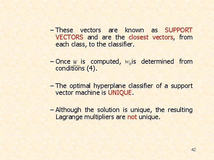
– These vectors are known as SUPPORT VECTORS and are the closest vectors, from each class, to the classifier. – Once is computed, conditions (4). is determined from – The optimal hyperplane classifier of a support vector machine is UNIQUE. – Although the solution is unique, the resulting Lagrange multipliers are not unique. 42

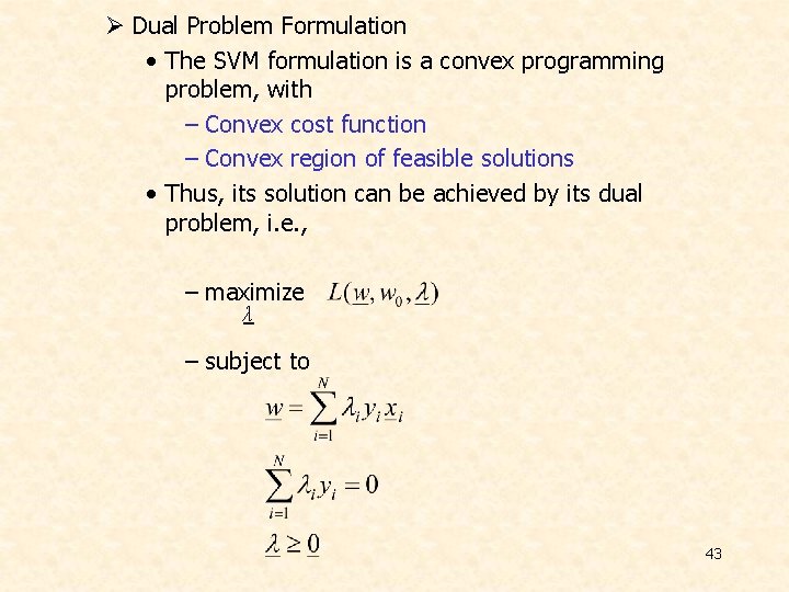
Ø Dual Problem Formulation • The SVM formulation is a convex programming problem, with – Convex cost function – Convex region of feasible solutions • Thus, its solution can be achieved by its dual problem, i. e. , – maximize λ – subject to 43

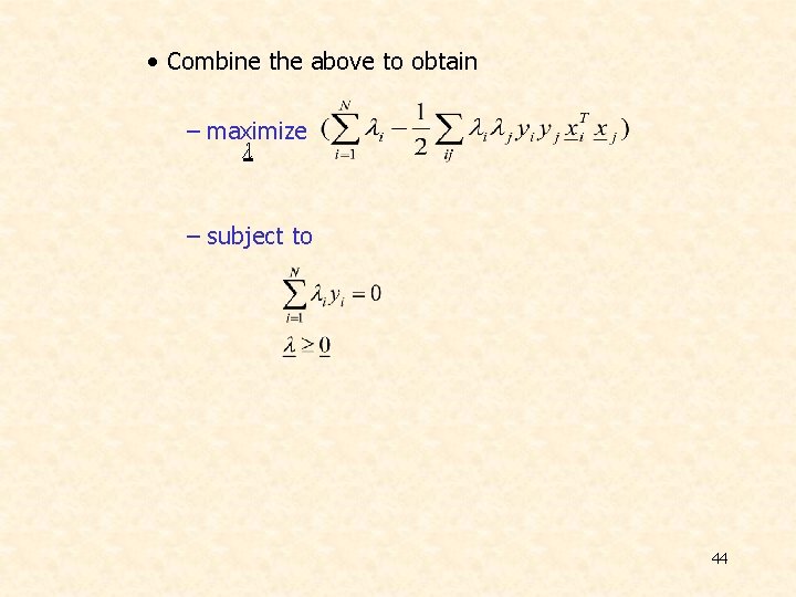
• Combine the above to obtain – maximize λ – subject to 44

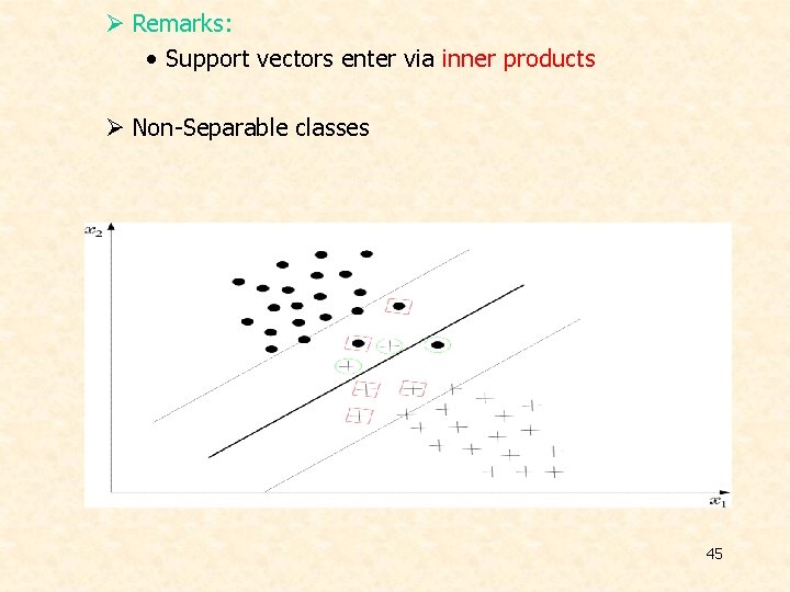
Ø Remarks: • Support vectors enter via inner products Ø Non-Separable classes 45

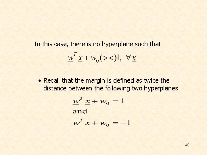
In this case, there is no hyperplane such that • Recall that the margin is defined as twice the distance between the following two hyperplanes 46

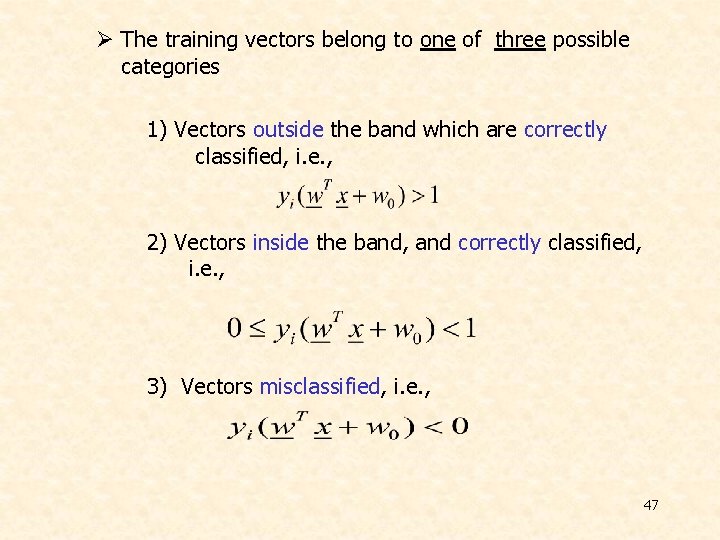
Ø The training vectors belong to one of three possible categories 1) Vectors outside the band which are correctly classified, i. e. , 2) Vectors inside the band, and correctly classified, i. e. , 3) Vectors misclassified, i. e. , 47

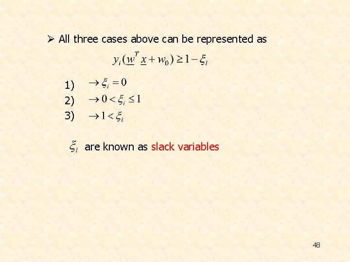
Ø All three cases above can be represented as 1) 2) 3) are known as slack variables 48

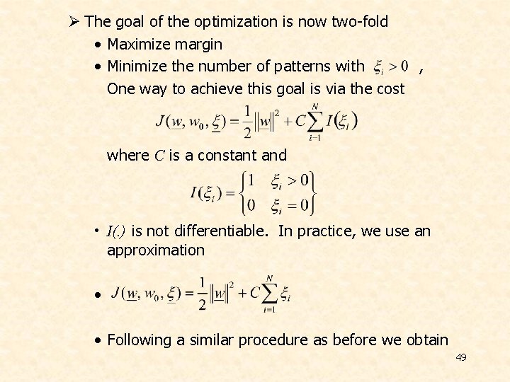
Ø The goal of the optimization is now two-fold • Maximize margin • Minimize the number of patterns with , One way to achieve this goal is via the cost where C is a constant and • I(. ) is not differentiable. In practice, we use an approximation • • Following a similar procedure as before we obtain 49

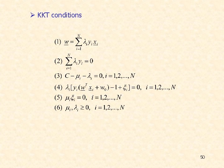
Ø KKT conditions 50

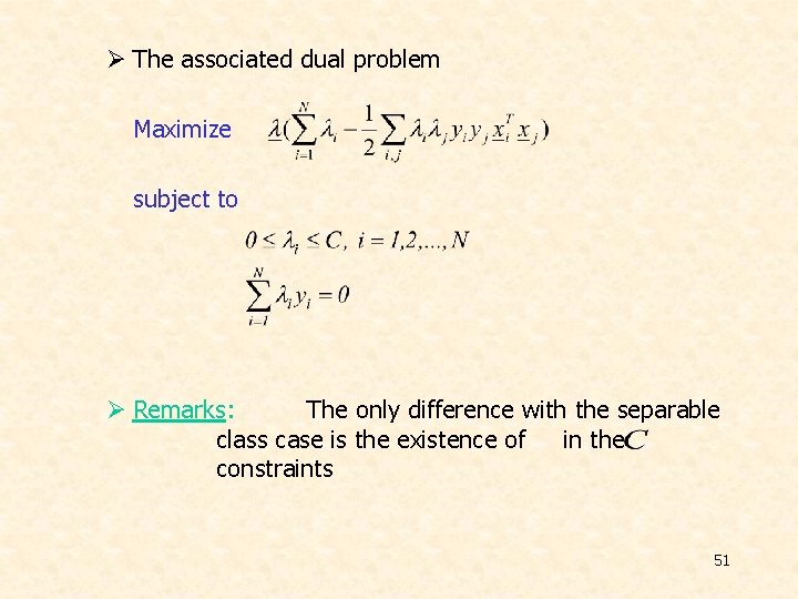
Ø The associated dual problem Maximize subject to Ø Remarks: The only difference with the separable class case is the existence of in the constraints 51

Ø Training the SVM A major problem is the high computational cost. To this end, decomposition techniques are used. The rationale behind them consists of the following: • Start with an arbitrary data subset (working set) that can fit in the memory. Perform optimization, via a general purpose optimizer. • Resulting support vectors remain in the working set, while others are replaced by new ones (outside the set) that violate severely the KKT conditions. • Repeat the procedure. • The above procedure guarantees that the cost function decreases. • Platt’s SMO algorithm chooses a working set of two samples, thus analytic optimization solution can be obtained. 52

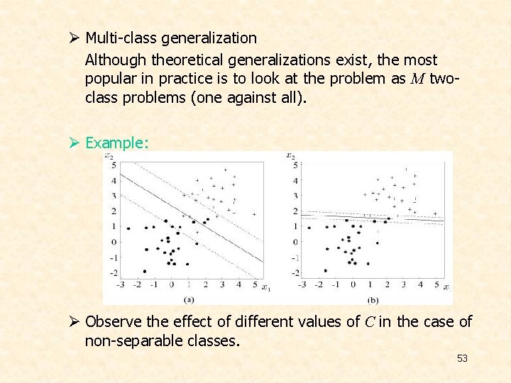
Ø Multi-class generalization Although theoretical generalizations exist, the most popular in practice is to look at the problem as M twoclass problems (one against all). Ø Example: Ø Observe the effect of different values of C in the case of non-separable classes. 53