Linear Arrays Representation Traversal Insertion Deletion Linear Search

Linear Arrays Representation & Traversal Insertion Deletion Linear Search Bubble Sort Binary Search

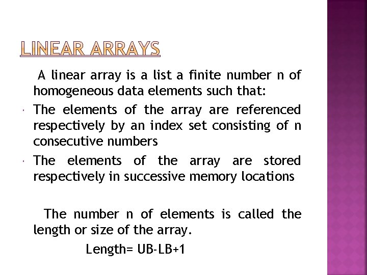
A linear array is a list a finite number n of homogeneous data elements such that: The elements of the array are referenced respectively by an index set consisting of n consecutive numbers The elements of the array are stored respectively in successive memory locations The number n of elements is called the length or size of the array. Length= UB-LB+1

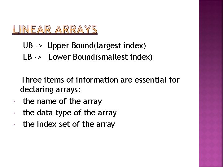
UB -> Upper Bound(largest index) LB -> Lower Bound(smallest index) Three items of information are essential for declaring arrays: the name of the array the data type of the array the index set of the array

Let LA be a linear array in the memory of the computer. LOC(LA[K])=address of the element LA[K] of the array LA 1000 1001 1002 1003 Computer Memory

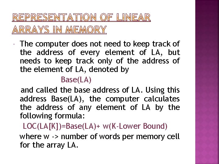
The computer does not need to keep track of the address of every element of LA, but needs to keep track only of the address of the element of LA, denoted by Base(LA) and called the base address of LA. Using this address Base(LA), the computer calculates the address of any element of LA by the following formula: LOC(LA[K])=Base(LA)+ w(K-Lower Bound) where w -> number of words per memory cell for the array LA.

Let A be a collection of data elements stored in memory of the computer. Suppose we want to print the contents of each element A or suppose we want to count the number of elements of A with a given property. This can be accomplished by traversing and processing each element of A exactly once.

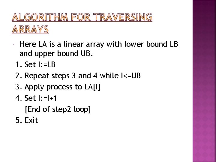
Here LA is a linear array with lower bound LB and upper bound UB. 1. Set I: =LB 2. Repeat steps 3 and 4 while I<=UB 3. Apply process to LA[I] 4. Set I: =I+1 [End of step 2 loop] 5. Exit

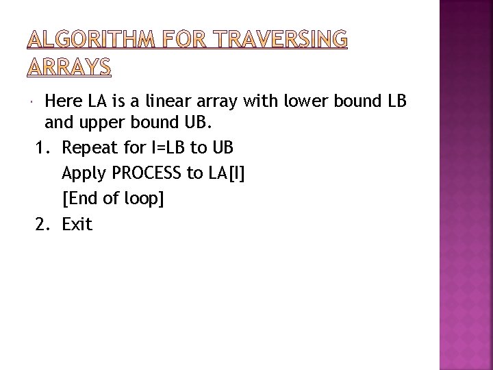
Here LA is a linear array with lower bound LB and upper bound UB. 1. Repeat for I=LB to UB Apply PROCESS to LA[I] [End of loop] 2. Exit

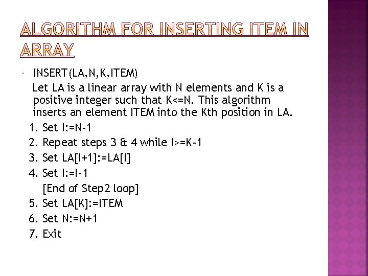
INSERT(LA, N, K, ITEM) Let LA is a linear array with N elements and K is a positive integer such that K<=N. This algorithm inserts an element ITEM into the Kth position in LA. 1. Set I: =N-1 2. Repeat steps 3 & 4 while I>=K-1 3. Set LA[I+1]: =LA[I] 4. Set I: =I-1 [End of Step 2 loop] 5. Set LA[K]: =ITEM 6. Set N: =N+1 7. Exit

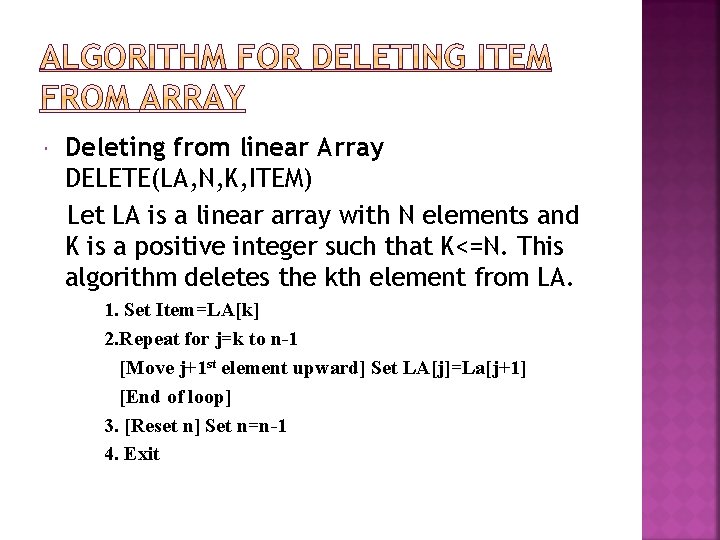
Deleting from linear Array DELETE(LA, N, K, ITEM) Let LA is a linear array with N elements and K is a positive integer such that K<=N. This algorithm deletes the kth element from LA. 1. Set Item=LA[k] 2. Repeat for j=k to n-1 [Move j+1 st element upward] Set LA[j]=La[j+1] [End of loop] 3. [Reset n] Set n=n-1 4. Exit

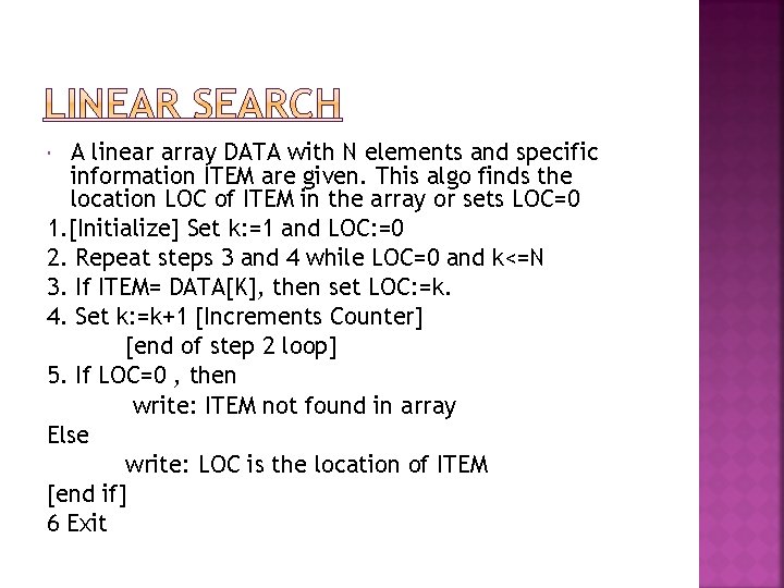
A linear array DATA with N elements and specific information ITEM are given. This algo finds the location LOC of ITEM in the array or sets LOC=0 1. [Initialize] Set k: =1 and LOC: =0 2. Repeat steps 3 and 4 while LOC=0 and k<=N 3. If ITEM= DATA[K], then set LOC: =k. 4. Set k: =k+1 [Increments Counter] [end of step 2 loop] 5. If LOC=0 , then write: ITEM not found in array Else write: LOC is the location of ITEM [end if] 6 Exit

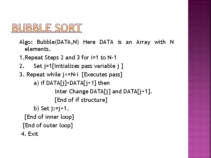
Algo: Bubble(DATA, N) Here DATA is an Array with N elements. 1. Repeat Steps 2 and 3 for i=1 to N-1 2. Set j=1[Initializes pass variable j ] 3. Repeat while j<=N-i [Executes pass] a) if DATA[j]>DATA[j+1] then Inter Change DATA[j] and DATA[j+1]. [End of if structure] b) Set j: =j+1. [End of inner loop] [End of outer loop] 4. Exit

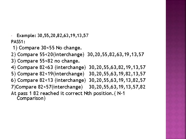
Example: 30, 55, 20, 82, 63, 19, 13, 57 PASS 1: 1) Compare 30<55 No change. 2) Compare 55<20(interchange) 30, 20, 55, 82, 63, 19, 13, 57 3) Compare 55<82 no change. 4) Compare 82<63 (interchange) 30, 20, 55, 63, 82, 19, 13, 57 5) Compare 82<19(interchange) 30, 20, 55, 63, 19, 82, 13, 57 6) Compare 82<13 (interchange) 30, 20, 55, 63, 19, 13, 82, 57 7)Compare 82<57(interchange) 30, 20, 55, 63, 19, 13, 57, 82 At pass 1 82 reached it correct Nth position. ( N-1 Comparison)

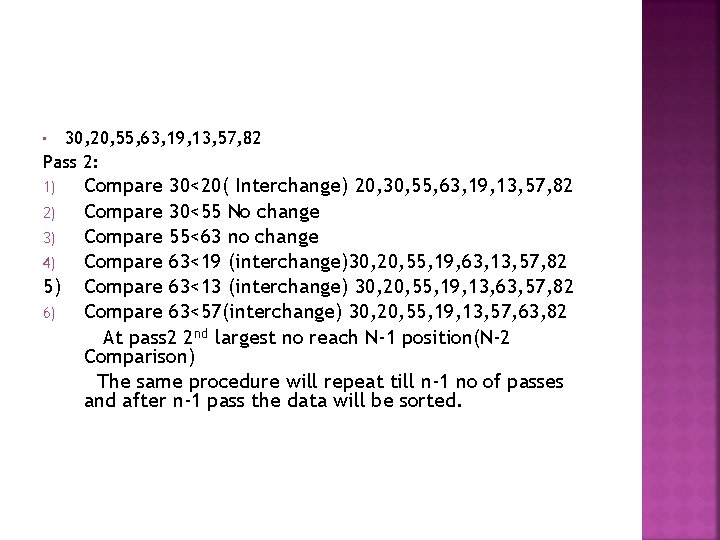
30, 20, 55, 63, 19, 13, 57, 82 Pass 2: • 1) 2) 3) 4) 5) 6) Compare 30<20( Interchange) 20, 30, 55, 63, 19, 13, 57, 82 Compare 30<55 No change Compare 55<63 no change Compare 63<19 (interchange)30, 20, 55, 19, 63, 13, 57, 82 Compare 63<13 (interchange) 30, 20, 55, 19, 13, 63, 57, 82 Compare 63<57(interchange) 30, 20, 55, 19, 13, 57, 63, 82 At pass 2 2 nd largest no reach N-1 position(N-2 Comparison) The same procedure will repeat till n-1 no of passes and after n-1 pass the data will be sorted.

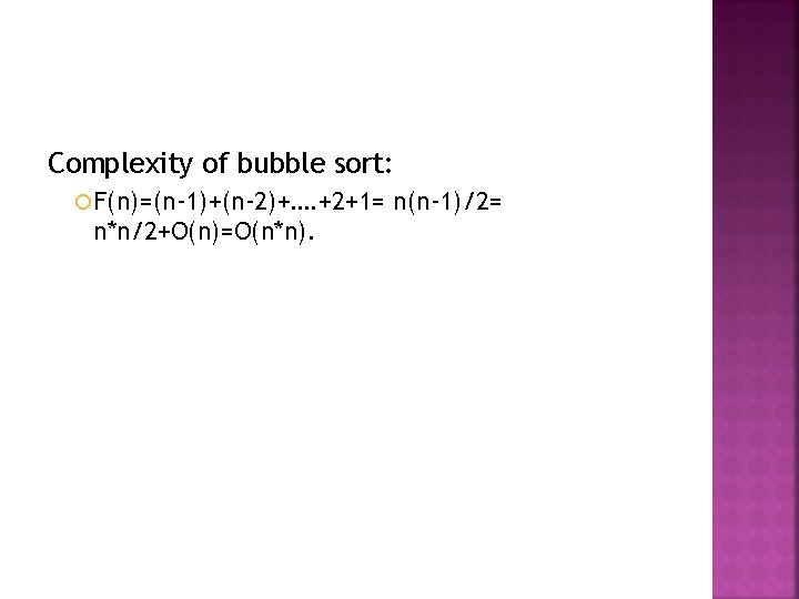
Complexity of bubble sort: F(n)=(n-1)+(n-2)+…. +2+1= n*n/2+O(n)=O(n*n). n(n-1)/2=

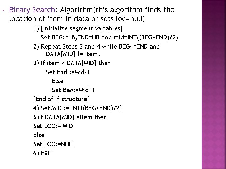
• Binary Search: Algorithm(this algorithm finds the location of item in data or sets loc=null) 1) [Initialize segment variables] Set BEG: =LB, END=UB and mid=INT((BEG+END)/2) 2) Repeat Steps 3 and 4 while BEG<=END and DATA[MID] != Item. 3) If item < DATA[MID] then Set End : =Mid-1 Else Set Beg: =Mid+1 [End of if structure] 4) Set MID : = INT((BEG+END)/2) 5)If DATA[MID] =Item then Set LOC: = MID Else Set LOC: =NULL 6) EXIT