Linear and anisotropic diffusion in image processing A

Linear and anisotropic diffusion in image processing: A study on implementation, parameters and segmentation Patricia van Marlen April 12, 2018 1

Outline Introduction Part 1: - diffusion filtering methods - numerical schemes - results: methods and schemes Part 2: - time step Δt: theory and results - stopping time S: theory and results Part 3: - results: segmentation Conclusion and further research 2

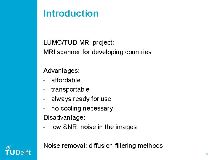
Introduction LUMC/TUD MRI project: MRI scanner for developing countries 3

Introduction LUMC/TUD MRI project: MRI scanner for developing countries Advantages: - affordable 4

Introduction LUMC/TUD MRI project: MRI scanner for developing countries Advantages: - affordable - transportable 5

Introduction LUMC/TUD MRI project: MRI scanner for developing countries Advantages: - affordable - transportable - always ready for use - no cooling necessary 6

Introduction LUMC/TUD MRI project: MRI scanner for developing countries Advantages: - affordable - transportable - always ready for use - no cooling necessary Disadvantage: - low SNR: noise in the images 7

Introduction LUMC/TUD MRI project: MRI scanner for developing countries Advantages: - affordable - transportable - always ready for use - no cooling necessary Disadvantage: - low SNR: noise in the images Noise removal: diffusion filtering methods 8

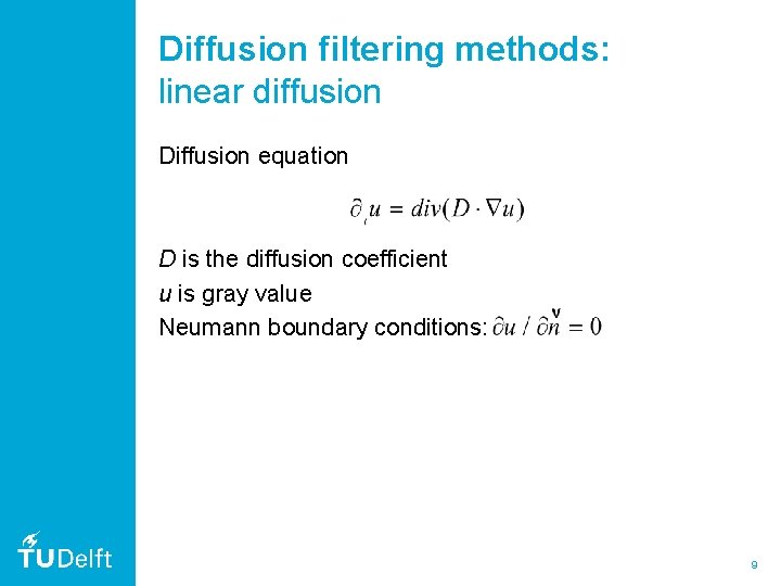
Diffusion filtering methods: linear diffusion Diffusion equation D is the diffusion coefficient u is gray value Neumann boundary conditions: 9

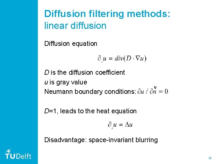
Diffusion filtering methods: linear diffusion Diffusion equation D is the diffusion coefficient u is gray value Neumann boundary conditions: D=1, leads to the heat equation Disadvantage: space-invariant blurring 10

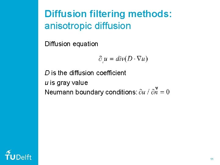
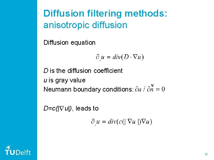
Diffusion filtering methods: anisotropic diffusion Diffusion equation D is the diffusion coefficient u is gray value Neumann boundary conditions: 11

Diffusion filtering methods: anisotropic diffusion Diffusion equation D is the diffusion coefficient u is gray value Neumann boundary conditions: D=c(| u|), leads to 12

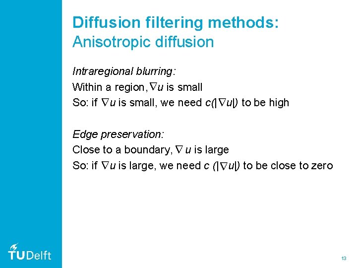
Diffusion filtering methods: Anisotropic diffusion Intraregional blurring: Within a region, u is small So: if u is small, we need c(| u|) to be high Edge preservation: Close to a boundary, u is large So: if u is large, we need c (| u|) to be close to zero 13

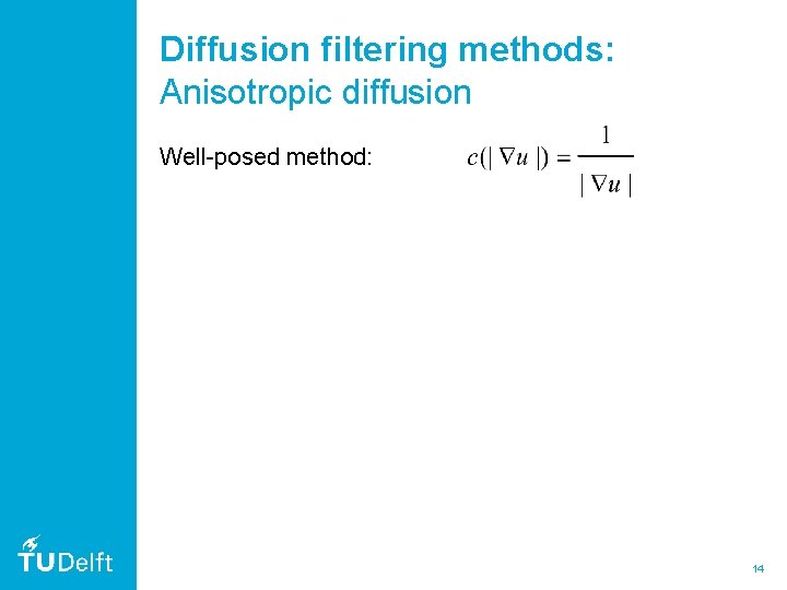
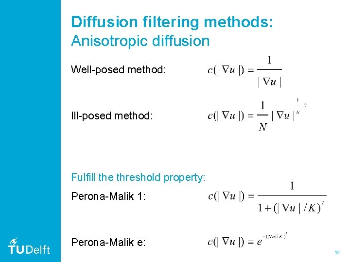
Diffusion filtering methods: Anisotropic diffusion Well-posed method: 14

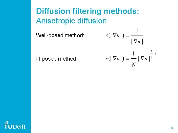
Diffusion filtering methods: Anisotropic diffusion Well-posed method: Ill-posed method: 15

Diffusion filtering methods: Anisotropic diffusion Well-posed method: Ill-posed method: Fulfill the threshold property: Perona-Malik 1: Perona-Malik e: 16

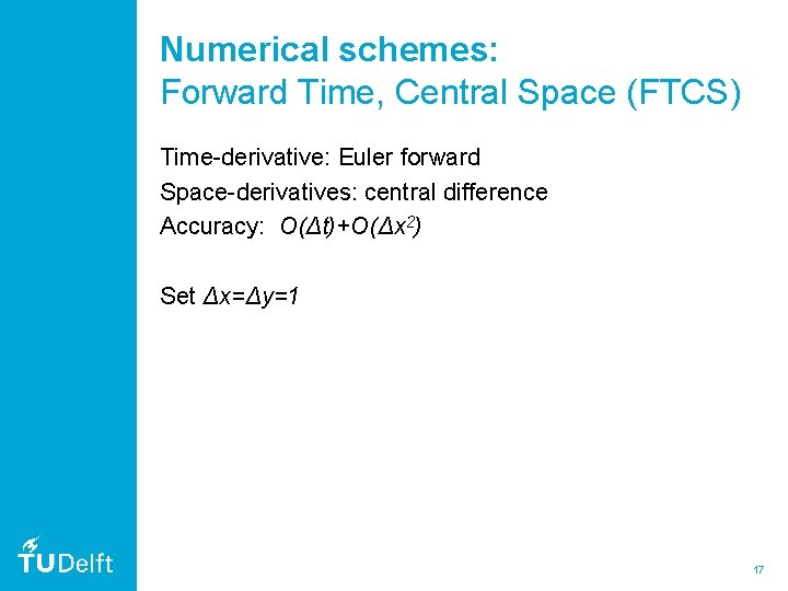
Numerical schemes: Forward Time, Central Space (FTCS) Time-derivative: Euler forward Space-derivatives: central difference Accuracy: O(Δt)+O(Δx 2) Set Δx=Δy=1 17

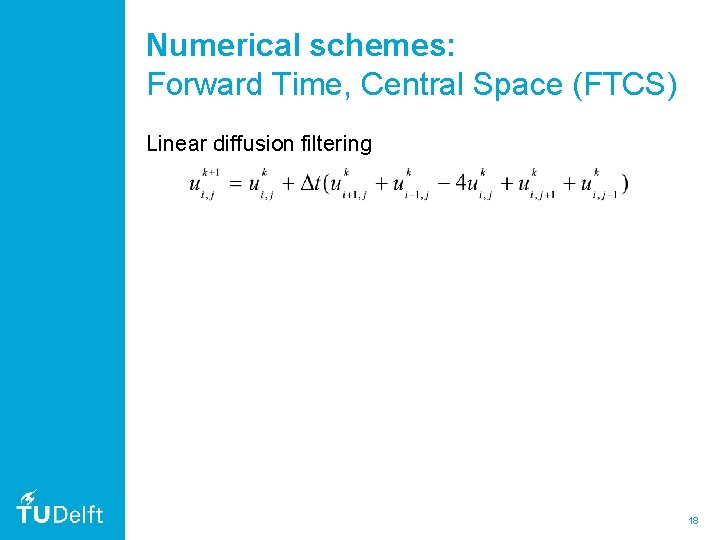
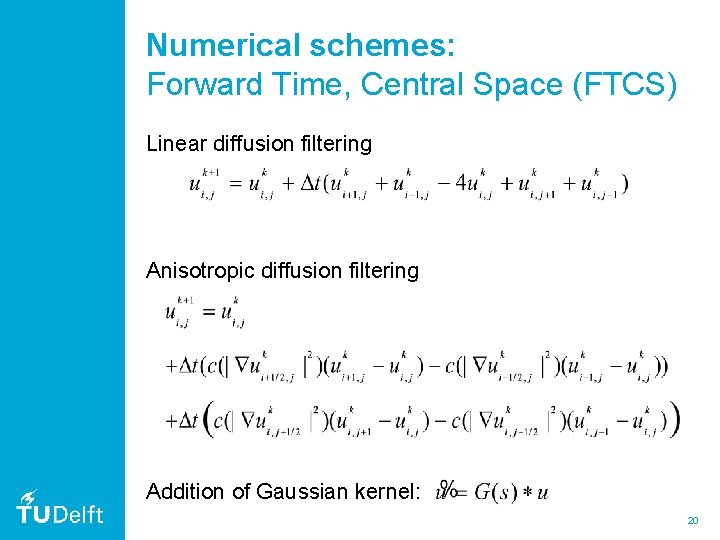
Numerical schemes: Forward Time, Central Space (FTCS) Linear diffusion filtering 18

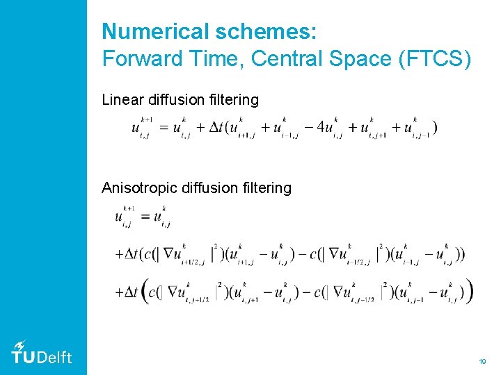
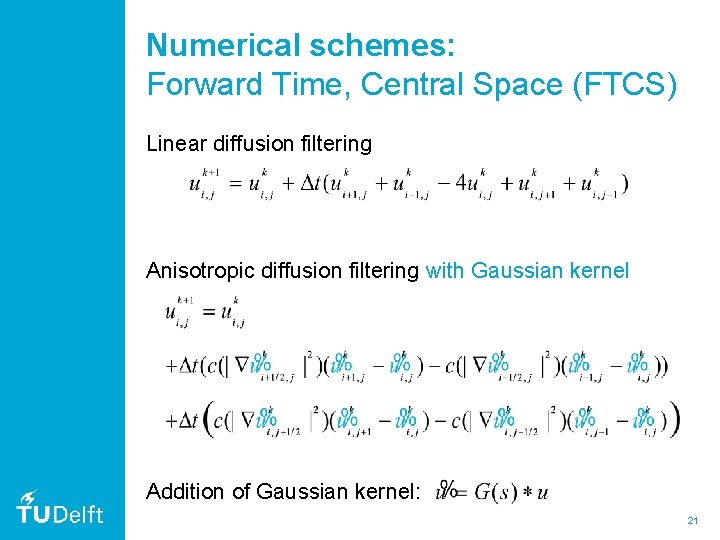
Numerical schemes: Forward Time, Central Space (FTCS) Linear diffusion filtering Anisotropic diffusion filtering 19

Numerical schemes: Forward Time, Central Space (FTCS) Linear diffusion filtering Anisotropic diffusion filtering Addition of Gaussian kernel: 20

Numerical schemes: Forward Time, Central Space (FTCS) Linear diffusion filtering Anisotropic diffusion filtering with Gaussian kernel Addition of Gaussian kernel: 21

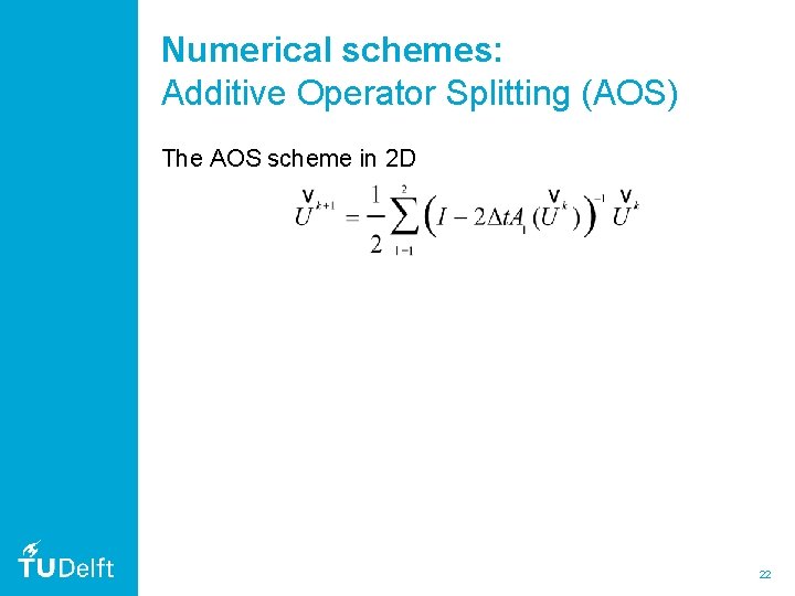
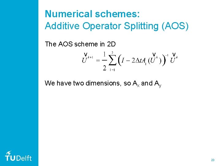
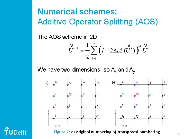
Numerical schemes: Additive Operator Splitting (AOS) The AOS scheme in 2 D 22

Numerical schemes: Additive Operator Splitting (AOS) The AOS scheme in 2 D We have two dimensions, so Ax and Ay 23

Numerical schemes: Additive Operator Splitting (AOS) The AOS scheme in 2 D We have two dimensions, so Ax and Ay Figure 2: a) original numbering b) transposed numbering 24

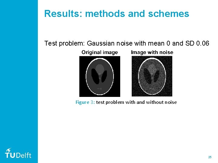
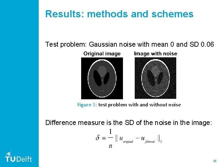
Results: methods and schemes Test problem: Gaussian noise with mean 0 and SD 0. 06 Figure 3: test problem with and without noise 25

Results: methods and schemes Test problem: Gaussian noise with mean 0 and SD 0. 06 Figure 3: test problem with and without noise Difference measure is the SD of the noise in the image: 26

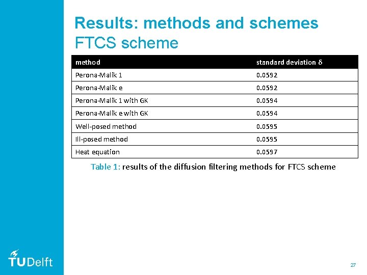
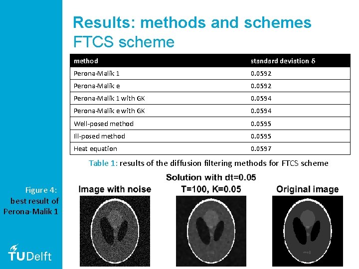
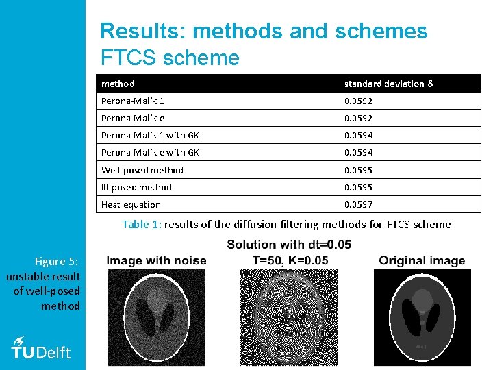
Results: methods and schemes FTCS scheme method standard deviation δ Perona-Malik 1 0. 0592 Perona-Malik e 0. 0592 Perona-Malik 1 with GK 0. 0594 Perona-Malik e with GK 0. 0594 Well-posed method 0. 0595 Ill-posed method 0. 0595 Heat equation 0. 0597 Table 1: results of the diffusion filtering methods for FTCS scheme 27

Results: methods and schemes FTCS scheme method standard deviation δ Perona-Malik 1 0. 0592 Perona-Malik e 0. 0592 Perona-Malik 1 with GK 0. 0594 Perona-Malik e with GK 0. 0594 Well-posed method 0. 0595 Ill-posed method 0. 0595 Heat equation 0. 0597 Table 1: results of the diffusion filtering methods for FTCS scheme Figure 4: best result of Perona-Malik 1 28

Results: methods and schemes FTCS scheme method standard deviation δ Perona-Malik 1 0. 0592 Perona-Malik e 0. 0592 Perona-Malik 1 with GK 0. 0594 Perona-Malik e with GK 0. 0594 Well-posed method 0. 0595 Ill-posed method 0. 0595 Heat equation 0. 0597 Table 1: results of the diffusion filtering methods for FTCS scheme Figure 5: unstable result of well-posed method 29

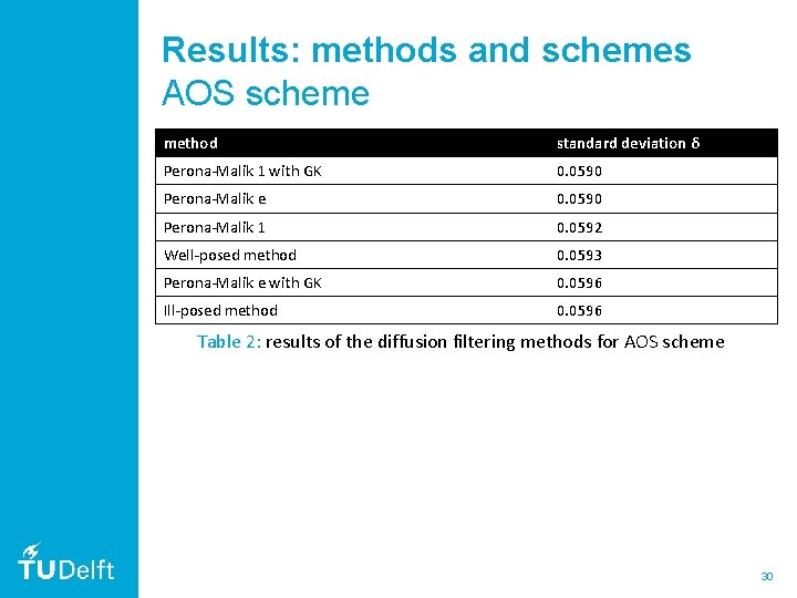
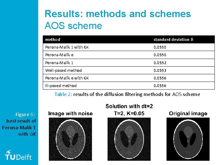
Results: methods and schemes AOS scheme method standard deviation δ Perona-Malik 1 with GK 0. 0590 Perona-Malik e 0. 0590 Perona-Malik 1 0. 0592 Well-posed method 0. 0593 Perona-Malik e with GK 0. 0596 Ill-posed method 0. 0596 Table 2: results of the diffusion filtering methods for AOS scheme 30

Results: methods and schemes AOS scheme method standard deviation δ Perona-Malik 1 with GK 0. 0590 Perona-Malik e 0. 0590 Perona-Malik 1 0. 0592 Well-posed method 0. 0593 Perona-Malik e with GK 0. 0596 Ill-posed method 0. 0596 Table 2: results of the diffusion filtering methods for AOS scheme Figure 6: best result of Perona-Malik 1 with GK 31

Results: methods and schemes conclusions - the AOS scheme gave slightly better results, but due to calculation time FTCS is used for the following parts 32

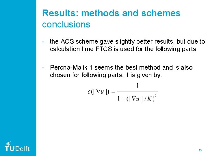
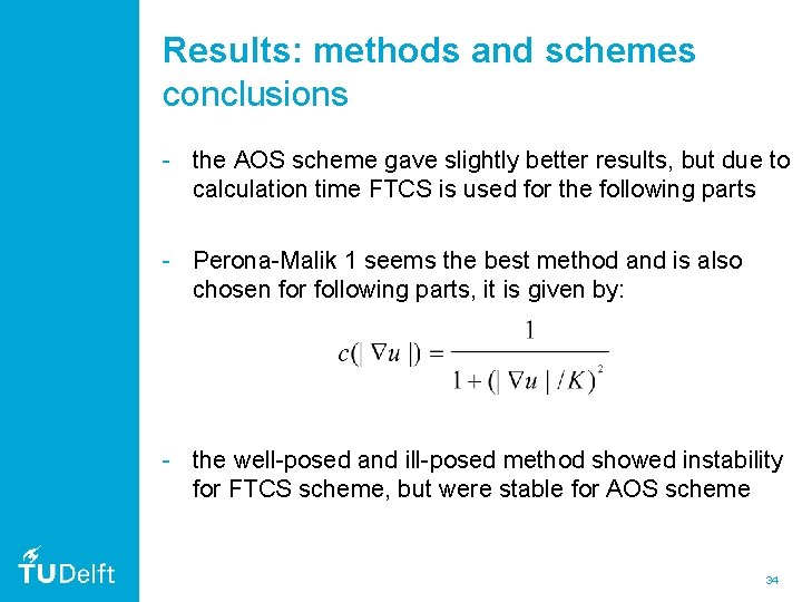
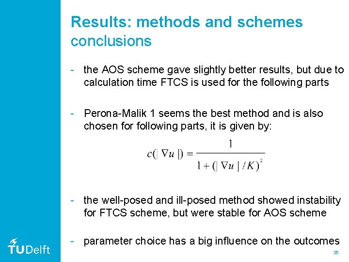
Results: methods and schemes conclusions - the AOS scheme gave slightly better results, but due to calculation time FTCS is used for the following parts - Perona-Malik 1 seems the best method and is also chosen for following parts, it is given by: 33

Results: methods and schemes conclusions - the AOS scheme gave slightly better results, but due to calculation time FTCS is used for the following parts - Perona-Malik 1 seems the best method and is also chosen for following parts, it is given by: - the well-posed and ill-posed method showed instability for FTCS scheme, but were stable for AOS scheme 34

Results: methods and schemes conclusions - the AOS scheme gave slightly better results, but due to calculation time FTCS is used for the following parts - Perona-Malik 1 seems the best method and is also chosen for following parts, it is given by: - the well-posed and ill-posed method showed instability for FTCS scheme, but were stable for AOS scheme - parameter choice has a big influence on the outcomes 35

Parameter study Investigation of - parameter K, used in the Perona-Malik functions - time step size Δt - number of time steps T 36

Parameter study Investigation of - parameter K, used in the Perona-Malik functions - time step size Δt - number of time steps T 37

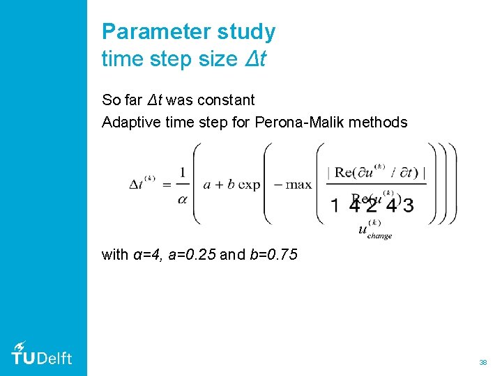
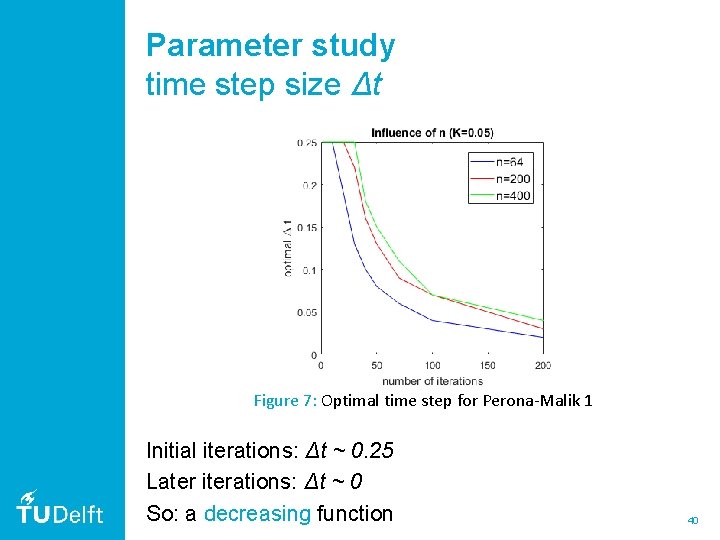
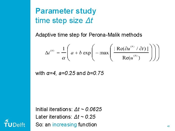
Parameter study time step size Δt So far Δt was constant Adaptive time step for Perona-Malik methods with α=4, a=0. 25 and b=0. 75 38

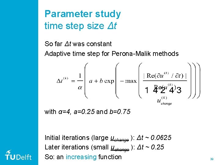
Parameter study time step size Δt So far Δt was constant Adaptive time step for Perona-Malik methods with α=4, a=0. 25 and b=0. 75 Initial iterations (large uchange ): Δt ~ 0. 0625 Later iterations (small uchange ): Δt ~ 0. 25 So: an increasing function 39

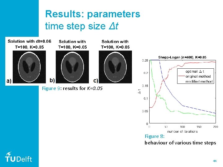
Parameter study time step size Δt Figure 7: Optimal time step for Perona-Malik 1 Initial iterations: Δt ~ 0. 25 Later iterations: Δt ~ 0 So: a decreasing function 40

Parameter study time step size Δt Adaptive time step for Perona-Malik methods with α=4, a=0. 25 and b=0. 75 Initial iterations: Δt ~ 0. 0625 Later iterations: Δt ~ 0. 25 So: an increasing function 41

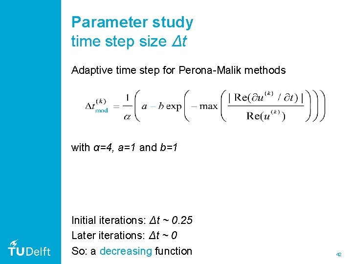
Parameter study time step size Δt Adaptive time step for Perona-Malik methods with α=4, a=1 and b=1 Initial iterations: Δt ~ 0. 25 Later iterations: Δt ~ 0 So: a decreasing function 42

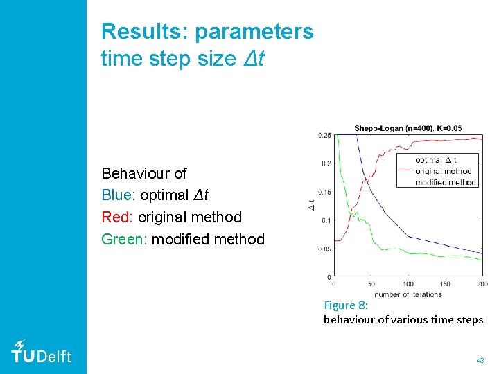
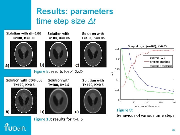
Results: parameters time step size Δt Behaviour of Blue: optimal Δt Red: original method Green: modified method Figure 8: behaviour of various time steps 43

Results: parameters time step size Δt Figure 9: results for K=0. 05 Figure 8: behaviour of various time steps 44

Results: parameters time step size Δt Figure 9: results for K=0. 05 Figure 10: results for K=0. 5 Figure 8: behaviour of various time steps 45

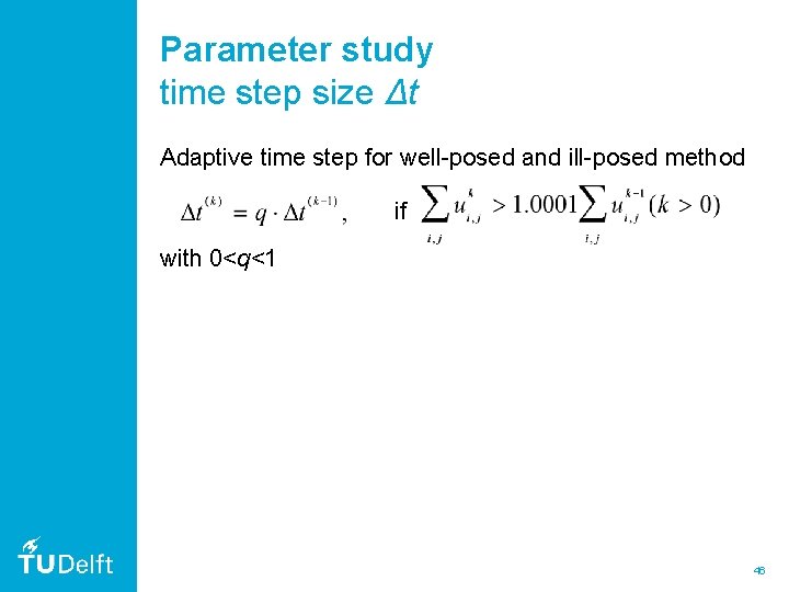
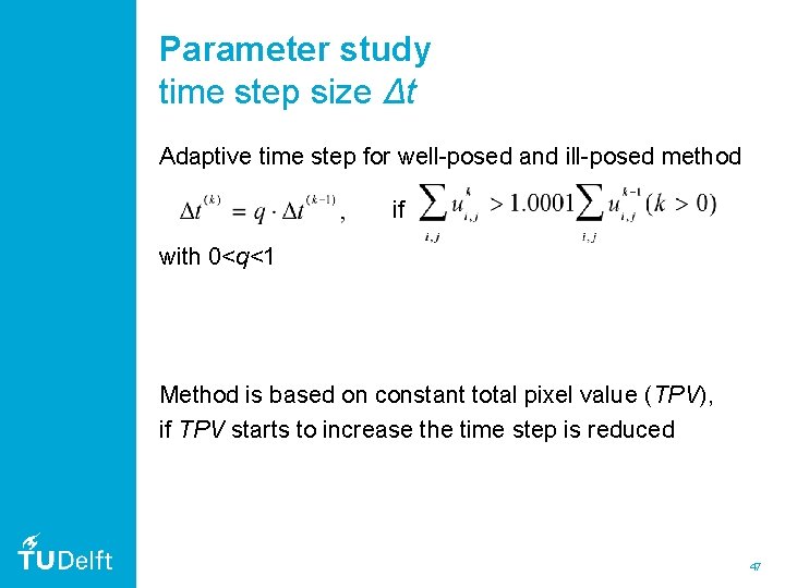
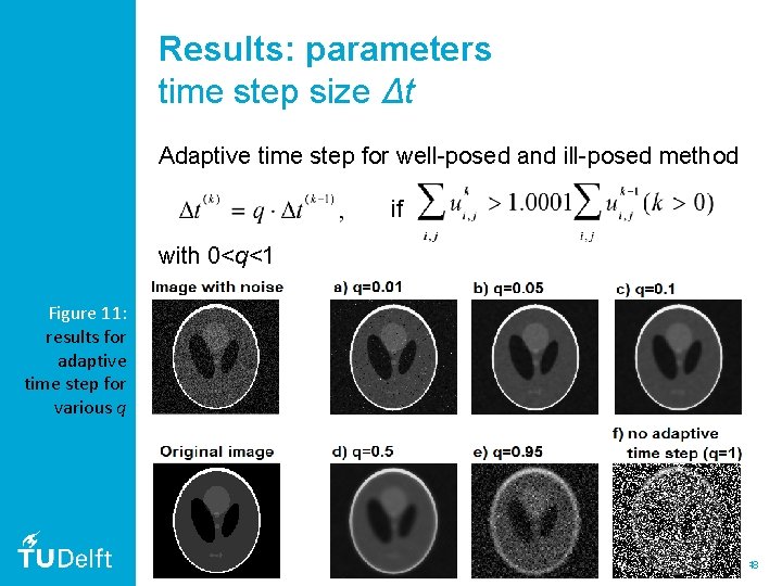
Parameter study time step size Δt Adaptive time step for well-posed and ill-posed method if with 0<q<1 46

Parameter study time step size Δt Adaptive time step for well-posed and ill-posed method if with 0<q<1 Method is based on constant total pixel value (TPV), if TPV starts to increase the time step is reduced 47

Results: parameters time step size Δt Adaptive time step for well-posed and ill-posed method if with 0<q<1 Figure 11: results for adaptive time step for various q 48

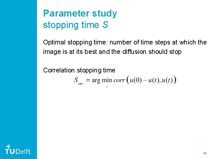
Parameter study stopping time S Optimal stopping time: number of time steps at which the image is at its best and the diffusion should stop 49

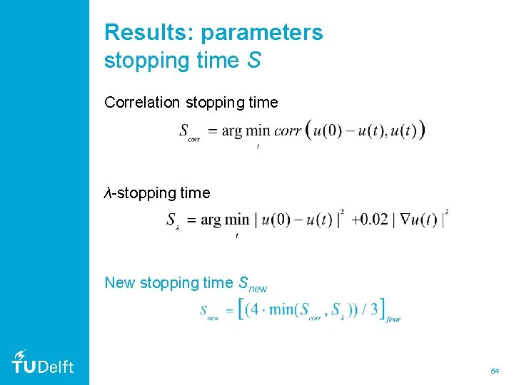
Parameter study stopping time S Optimal stopping time: number of time steps at which the image is at its best and the diffusion should stop Correlation stopping time 50

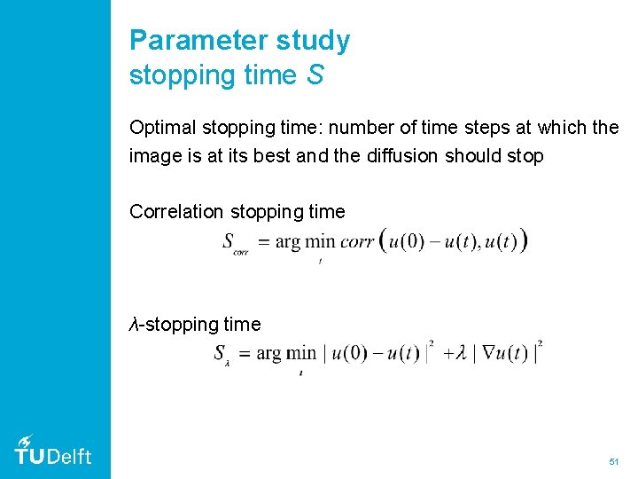
Parameter study stopping time S Optimal stopping time: number of time steps at which the image is at its best and the diffusion should stop Correlation stopping time λ-stopping time 51

Parameter study stopping time S Optimal stopping time: number of time steps at which the image is at its best and the diffusion should stop Correlation stopping time λ-stopping time 52

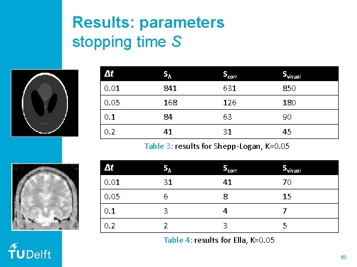
Results: parameters stopping time S Δt Sλ Scorr Svisual 0. 01 841 631 850 0. 05 168 126 180 0. 1 84 63 90 0. 2 41 31 45 Table 3: results for Shepp-Logan, K=0. 05 Δt Sλ Scorr Svisual 0. 01 31 41 70 0. 05 6 8 15 0. 1 3 4 7 0. 2 2 3 5 Table 4: results for Ella, K=0. 05 53

Results: parameters stopping time S Correlation stopping time λ-stopping time New stopping time Snew 54

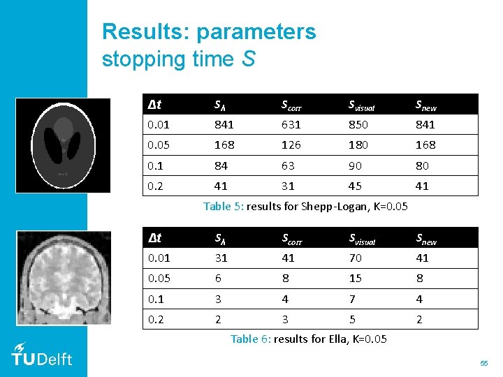
Results: parameters stopping time S Δt Sλ Scorr Svisual Snew 0. 01 841 631 850 841 0. 05 168 126 180 168 0. 1 84 63 90 80 0. 2 41 31 45 41 Table 5: results for Shepp-Logan, K=0. 05 Δt Sλ Scorr Svisual Snew 0. 01 31 41 70 41 0. 05 6 8 15 8 0. 1 3 4 7 4 0. 2 2 3 5 2 Table 6: results for Ella, K=0. 05 55

Results: parameters stopping time S Δt Sλ Scorr Svisual Snew 0. 01 841 631 850 841 0. 05 168 126 180 168 0. 1 84 63 90 80 0. 2 41 31 45 41 Table 5: results for Shepp-Logan, K=0. 05 Δt Sλ Scorr Svisual Snew 0. 01 31 41 70 41 0. 05 6 8 15 8 0. 1 3 4 7 4 0. 2 2 3 5 2 Table 6: results for Ella, K=0. 05 56

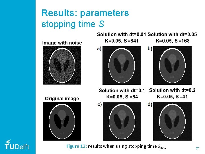
Results: parameters stopping time S Figure 12: results when using stopping time Snew 57

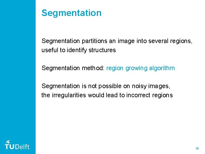
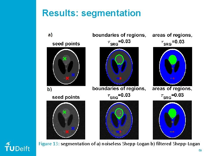
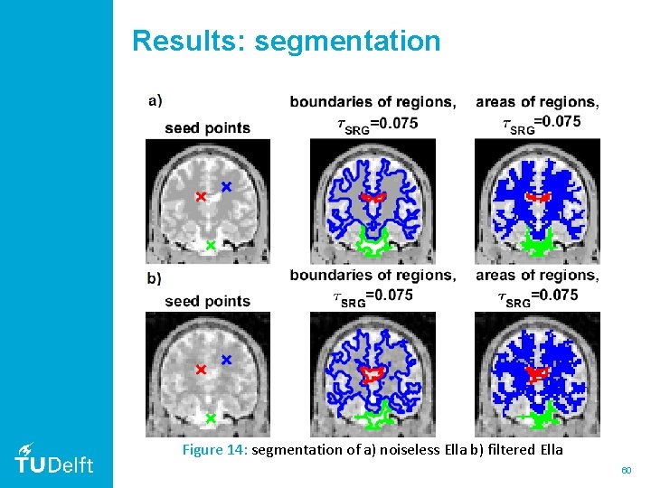
Segmentation partitions an image into several regions, useful to identify structures Segmentation method: region growing algorithm Segmentation is not possible on noisy images, the irregularities would lead to incorrect regions 58

Results: segmentation Figure 13: segmentation of a) noiseless Shepp-Logan b) filtered Shepp-Logan 59

Results: segmentation Figure 14: segmentation of a) noiseless Ella b) filtered Ella 60

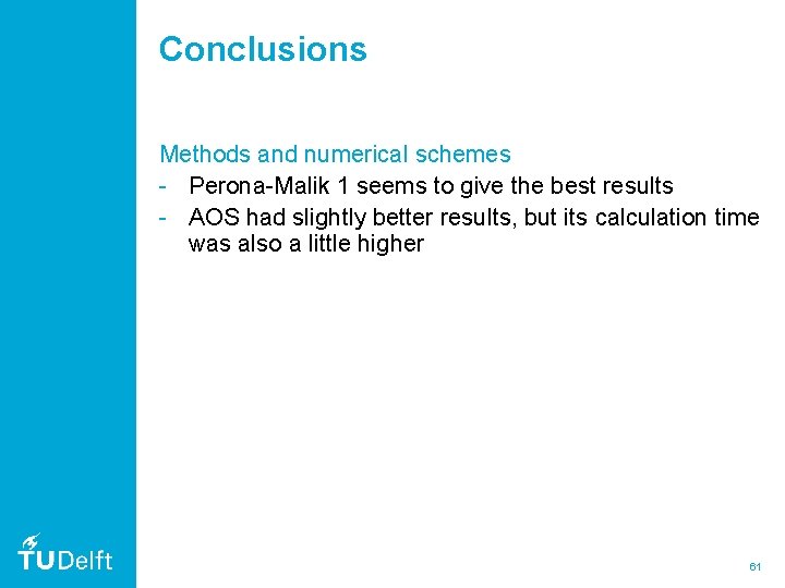
Conclusions Methods and numerical schemes - Perona-Malik 1 seems to give the best results - AOS had slightly better results, but its calculation time was also a little higher Parameter study introduced time step and stopping time lead to good results well-posed and ill-posed method were unstable for FTCS scheme, this can be overcome with an adaptive time step Segmentation showed that images obtained with anisotropic diffusion filtering are of good quality 61

Conclusions Methods and numerical schemes - Perona-Malik 1 seems to give the best results - AOS had slightly better results, but its calculation time was also a little higher Parameter study - introduced time step and stopping time lead to good results - well-posed and ill-posed method were unstable for FTCS scheme, this can be overcome with an adaptive time step Segmentation showed that images obtained with anisotropic diffusion filtering are of good quality 62

Conclusions Methods and numerical schemes - Perona-Malik 1 seems to give the best results - AOS had slightly better results, but its calculation time was also a little higher Parameter study - introduced time step and stopping time lead to good results - well-posed and ill-posed method were unstable for FTCS scheme, this can be overcome with an adaptive time step Segmentation - segmentation showed that images obtained with anisotropic diffusion filtering are of good quality 63

Further research - further investigation of parameters 64

Further research - further investigation of parameters - improve the calculation time of the AOS method 65

Further research - further investigation of parameters - improve the calculation time of the AOS method - test methods on real data 66

Questions? 67

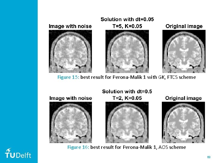
Figure 15: best result for Perona-Malik 1 with GK, FTCS scheme Figure 16: best result for Perona-Malik 1, AOS scheme 68

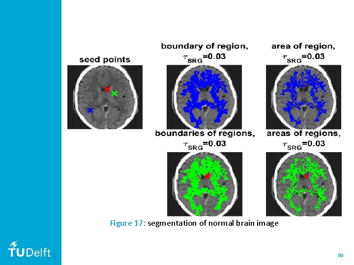
Figure 17: segmentation of normal brain image 69

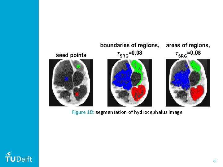
Figure 18: segmentation of hydrocephalus image 70