Linear Algebraic Graph Algorithms for Back End Processing

Linear Algebraic Graph Algorithms for Back End Processing Jeremy Kepner, Nadya Bliss, and Eric Robinson MIT Lincoln Laboratory This work is sponsored by the Department of Defense under Air Force Contract FA 8721 -05 -C-0002. Opinions, interpretations, conclusions, and recommendations are those of the author and are not necessarily endorsed by the United States Government. MIT Lincoln Laboratory Slide-1

Outline • Introduction • Power Law Graphs • Graph Benchmark • Results • Summary • Post Detection Processing • Sparse Matrix Duality • Approach MIT Lincoln Laboratory Slide-2

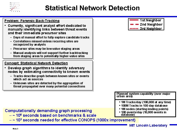
Statistical Network Detection 1 st Neighbor 2 nd Neighbor 3 rd Neighbor Problem: Forensic Back-Tracking • Currently, significant analyst effort dedicated to manually identifying links between threat events and their immediate precursor sites – Days of manual effort to fully explore candidate tracks – Correlations missed unless recurring sites are recognized by analysts – Precursor sites may be low-value staging areas – Manual analysis will not support further backtracking from staging areas to potentially higher-value sites Event B Concept: Statistical Network Detection • Develop graph algorithms to identify adversary nodes by estimating connectivity to known events – Tracks describe graph between known sites or events which act as sources – Unknown sites are detected by the aggregation of threat propagated over many potential connections Event A Planned system capability (over major urban area) • 1 M Tracks/day (100, 000 at any time) • 100 M Tracks in 100 day database • 1 M nodes (starting/ending points) • 100 events/day (10, 000 events in Computationally demanding graph processing database) – ~ 106 seconds based on benchmarks & scale – ~ 103 seconds needed for effective CONOPS (1000 x improvement) MIT Lincoln Laboratory Slide-3

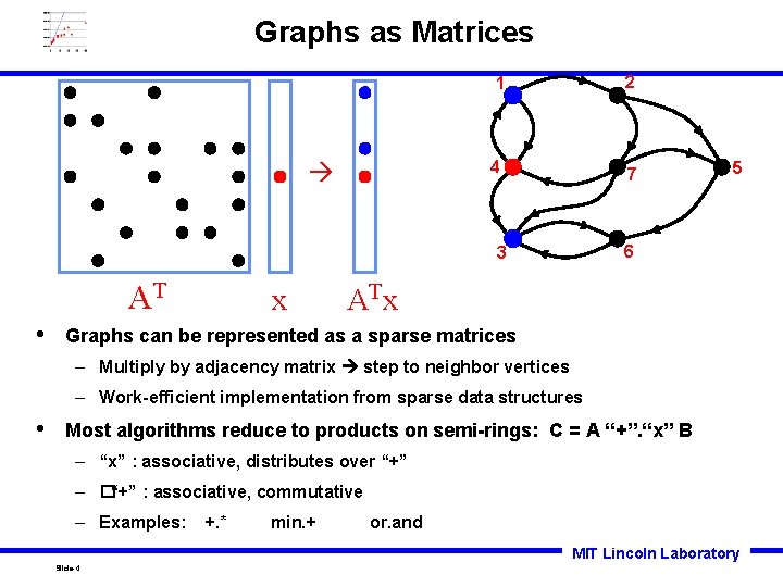
Graphs as Matrices 1 2 4 7 6 3 AT • x 5 AT x Graphs can be represented as a sparse matrices – Multiply by adjacency matrix step to neighbor vertices – Work-efficient implementation from sparse data structures • Most algorithms reduce to products on semi-rings: C = A “+”. “x” B – “x” : associative, distributes over “+” – �“+” : associative, commutative – Examples: +. * min. + or. and MIT Lincoln Laboratory Slide-4

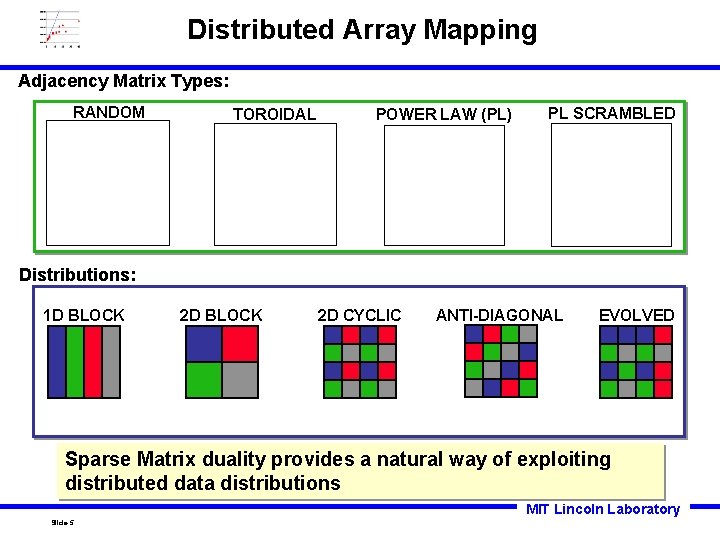
Distributed Array Mapping Adjacency Matrix Types: RANDOM TOROIDAL POWER LAW (PL) PL SCRAMBLED Distributions: 1 D BLOCK 2 D CYCLIC ANTI-DIAGONAL EVOLVED Sparse Matrix duality provides a natural way of exploiting distributed data distributions MIT Lincoln Laboratory Slide-5

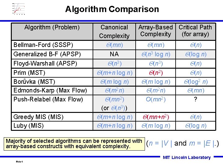
Algorithm Comparison Algorithm (Problem) Bellman-Ford (SSSP) Generalized B-F (APSP) Floyd-Warshall (APSP) Prim (MST) Borůvka (MST) Edmonds-Karp (Max Flow) Push-Relabel (Max Flow) Greedy MIS (MIS) Luby (MIS) Canonical Complexity (mn) NA (n 3) (m+n log n) (m 2 n) (mn 2) (or (n 3)) (m+n log n) Array-Based Critical Path Complexity (for array) (mn) (n 3 log n) (n 3) (n 2) (m log n) (m 2 n) (log n) (n) (log 2 n) (mn) O(mn 2) ? (mn+n 2) (m log n) (n) Majority of selected algorithms can be represented with array-based constructs with equivalent complexity. (log n) (n = |V | and m = |E |. ) MIT Lincoln Laboratory Slide-6

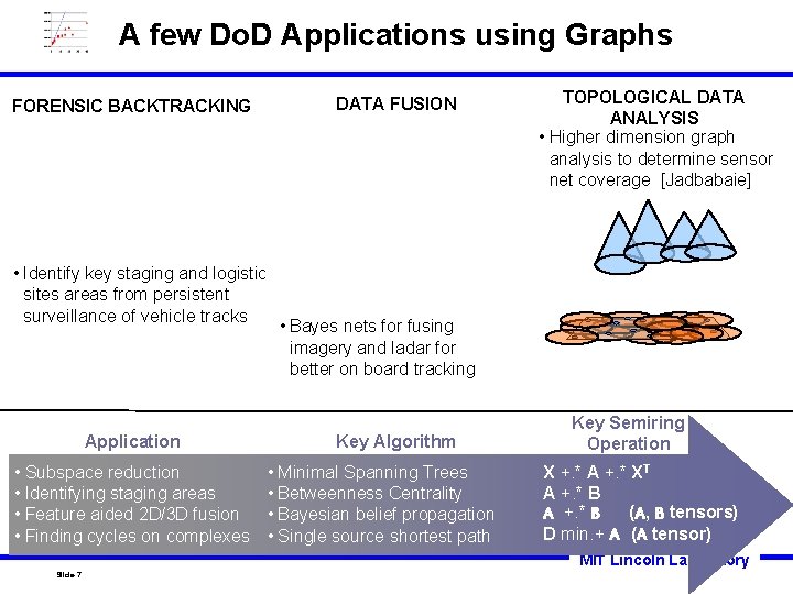
A few Do. D Applications using Graphs FORENSIC BACKTRACKING DATA FUSION Event B Event A • Identify key staging and logistic sites areas from persistent surveillance of vehicle tracks Application • Subspace reduction • Identifying staging areas • Feature aided 2 D/3 D fusion • Finding cycles on complexes TOPOLOGICAL DATA ANALYSIS • Higher dimension graph analysis to determine sensor net coverage [Jadbabaie] 2 D/3 D Fused Imagery • Bayes nets for fusing imagery and ladar for better on board tracking Key Algorithm • Minimal Spanning Trees • Betweenness Centrality • Bayesian belief propagation • Single source shortest path Key Semiring Operation X +. * A +. * XT A +. * B (A, B tensors) D min. + A (A tensor) MIT Lincoln Laboratory Slide-7

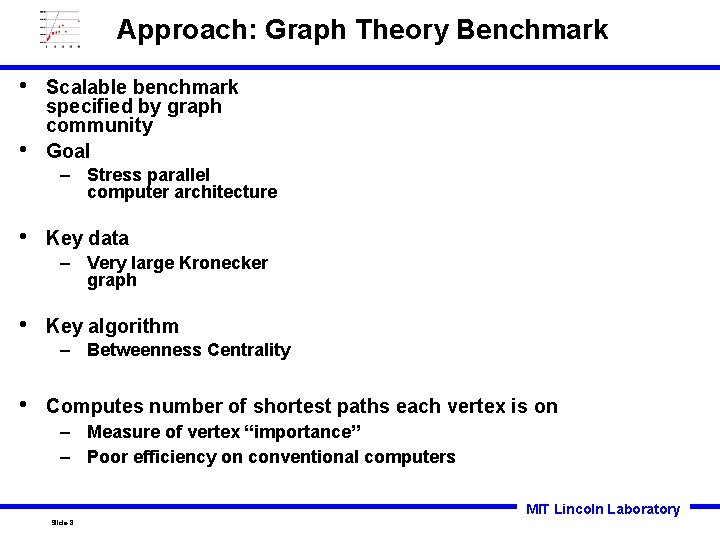
Approach: Graph Theory Benchmark • • Scalable benchmark specified by graph community Goal – Stress parallel computer architecture • Key data – Very large Kronecker graph • Key algorithm – Betweenness Centrality • Computes number of shortest paths each vertex is on – Measure of vertex “importance” – Poor efficiency on conventional computers MIT Lincoln Laboratory Slide-8

Outline • Introduction • Power Law Graphs • Graph Benchmark • Results • Summary • Kronecker Model • Analytic Results MIT Lincoln Laboratory Slide-9

Power Law Graphs Social Network Analysis Target Identification • • • Anomaly Detection Many graph algorithms must operate on power law graphs Most nodes have a few edges A few nodes have many edges MIT Lincoln Laboratory Slide-10

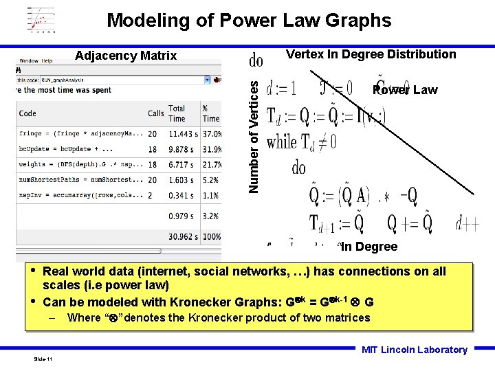
Modeling of Power Law Graphs Vertex In Degree Distribution Number of Vertices Adjacency Matrix Power Law In Degree • • Real world data (internet, social networks, …) has connections on all scales (i. e power law) Can be modeled with Kronecker Graphs: G k = G k-1 G – Where “ ”denotes the Kronecker product of two matrices MIT Lincoln Laboratory Slide-11

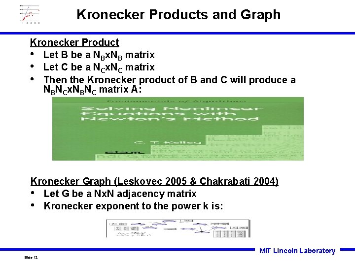
Kronecker Products and Graph Kronecker Product • Let B be a NBx. NB matrix • Let C be a NCx. NC matrix • Then the Kronecker product of B and C will produce a NBNCx. NBNC matrix A: Kronecker Graph (Leskovec 2005 & Chakrabati 2004) • Let G be a Nx. N adjacency matrix • Kronecker exponent to the power k is: MIT Lincoln Laboratory Slide-12

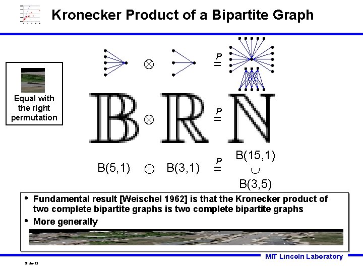
Kronecker Product of a Bipartite Graph Equal with the right permutation B(5, 1) • • P = B(3, 1) P = B(15, 1) B(3, 5) Fundamental result [Weischel 1962] is that the Kronecker product of two complete bipartite graphs is two complete bipartite graphs More generally MIT Lincoln Laboratory Slide-13

Degree Distribution of Bipartite Kronecker Graphs • Kronecker exponent of a bipartite graph produces many independent bipartite graphs • Only k+1 different kinds of nodes in this graph, with degree distribution MIT Lincoln Laboratory Slide-14

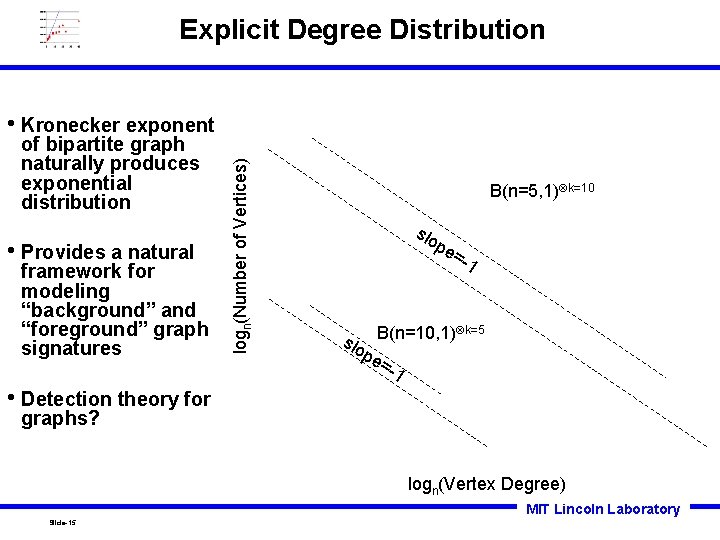
Explicit Degree Distribution of bipartite graph naturally produces exponential distribution • Provides a natural framework for modeling “background” and “foreground” graph signatures logn(Number of Vertices) • Kronecker exponent B(n=5, 1) k=10 slo pe =-1 k=5 slo B(n=10, 1) pe =-1 • Detection theory for graphs? logn(Vertex Degree) MIT Lincoln Laboratory Slide-15

Reference • Book: “Graph Algorithms in the Language of • • Linear Algebra” Editors: Kepner (MIT-LL) and Gilbert (UCSB) Contributors – Bader (Ga Tech) – Chakrabart (CMU) – Dunlavy (Sandia) – Faloutsos (CMU) – Fineman (MIT-LL & MIT) – Gilbert (UCSB) – Kahn (MIT-LL & Brown) – Kegelmeyer (Sandia) – Kepner (MIT-LL) – Kleinberg (Cornell) – Kolda (Sandia) – Leskovec (CMU) – Madduri (Ga Tech) – Robinson (MIT-LL & NEU), Shah (UCSB) Graph Algorithms in the Language of Linear Algebra Jeremy Kepner and John Gilbert (editors) MIT Lincoln Laboratory Slide-16

Outline • Introduction • Power Law Graphs • Graph Benchmark • Results • Summary • Post Detection Processing • Sparse Matrix Duality • Approach MIT Lincoln Laboratory Slide-17

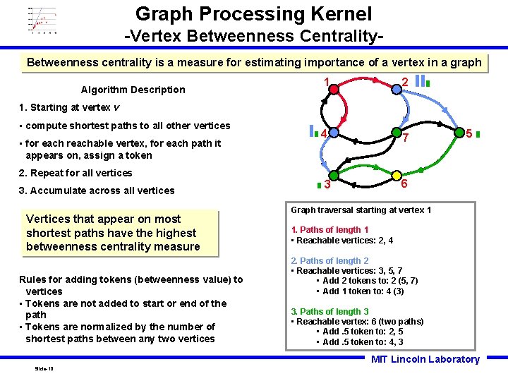
Graph Processing Kernel -Vertex Betweenness Centrality. Betweenness centrality is a measure for estimating importance of a vertex in a graph Algorithm Description 1 2 4 7 1. Starting at vertex v • compute shortest paths to all other vertices • for each reachable vertex, for each path it appears on, assign a token 2. Repeat for all vertices 3. Accumulate across all vertices Vertices that appear on most shortest paths have the highest betweenness centrality measure Rules for adding tokens (betweenness value) to vertices • Tokens are not added to start or end of the path • Tokens are normalized by the number of shortest paths between any two vertices 5 6 3 Graph traversal starting at vertex 1 1. Paths of length 1 • Reachable vertices: 2, 4 2. Paths of length 2 • Reachable vertices: 3, 5, 7 • Add 2 tokens to: 2 (5, 7) • Add 1 token to: 4 (3) 3. Paths of length 3 • Reachable vertex: 6 (two paths) • Add. 5 token to: 2, 5 • Add. 5 token to: 4, 3 MIT Lincoln Laboratory Slide-18

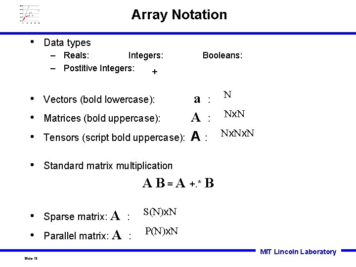
Array Notation • Data types – Reals: Integers: – Postitive Integers: + • Vectors (bold lowercase): • Matrices (bold uppercase): • Tensors (script bold uppercase): • Standard matrix multiplication Booleans: a : A: N Nx. Nx. N A B = A +. * B • Sparse matrix: A : S(N)x. N • Parallel matrix: A : P(N)x. N MIT Lincoln Laboratory Slide-19

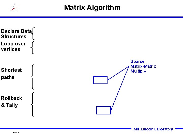
Matrix Algorithm Declare Data Structures Loop over vertices Shortest paths Sparse Matrix-Matrix Multiply Rollback & Tally MIT Lincoln Laboratory Slide-20

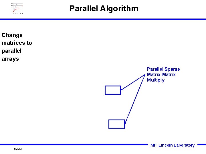
Parallel Algorithm Change matrices to parallel arrays Parallel Sparse Matrix-Matrix Multiply MIT Lincoln Laboratory Slide-21

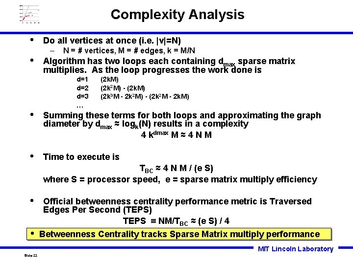
Complexity Analysis • • Do all vertices at once (i. e. |v|=N) – N = # vertices, M = # edges, k = M/N Algorithm has two loops each containing dmax sparse matrix multiplies. As the loop progresses the work done is d=1 d=2 d=3 … (2 k. M) (2 k 2 M) - (2 k. M) (2 k 3 M - 2 k 2 M) - (2 k 2 M - 2 k. M) • Summing these terms for both loops and approximating the graph diameter by dmax ≈ logk(N) results in a complexity 4 kdmax M ≈ 4 N M • Time to execute is TBC ≈ 4 N M / (e S) where S = processor speed, e = sparse matrix multiply efficiency • • Official betweenness centrality performance metric is Traversed Edges Per Second (TEPS) TEPS NM/TBC ≈ (e S) / 4 Betweenness Centrality tracks Sparse Matrix multiply performance MIT Lincoln Laboratory Slide-22

Outline • Introduction • Power Law Graphs • Graph Benchmark • Results • Summary • Post Detection Processing • Sparse Matrix Duality • Approach MIT Lincoln Laboratory Slide-23

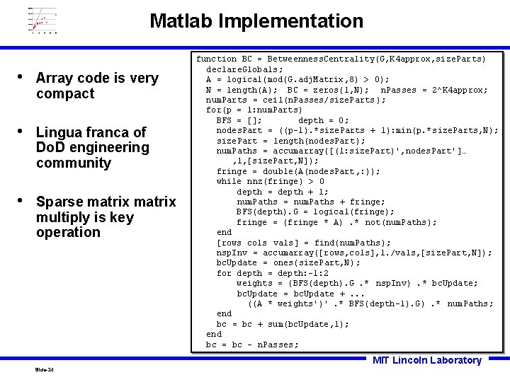
Matlab Implementation • Array code is very compact • Lingua franca of Do. D engineering community • Sparse matrix multiply is key operation function BC = Betweenness. Centrality(G, K 4 approx, size. Parts) declare. Globals; A = logical(mod(G. adj. Matrix, 8) > 0); N = length(A); BC = zeros(1, N); n. Passes = 2^K 4 approx; num. Parts = ceil(n. Passes/size. Parts); for(p = 1: num. Parts) BFS = []; depth = 0; nodes. Part = ((p-1). *size. Parts + 1): min(p. *size. Parts, N); size. Part = length(nodes. Part); num. Paths = accumarray([(1: size. Part)', nodes. Part']… , 1, [size. Part, N]); fringe = double(A(nodes. Part, : )); while nnz(fringe) > 0 depth = depth + 1; num. Paths = num. Paths + fringe; BFS(depth). G = logical(fringe); fringe = (fringe * A). * not(num. Paths); end [rows cols vals] = find(num. Paths); nsp. Inv = accumarray([rows, cols], 1. /vals, [size. Part, N]); bc. Update = ones(size. Part, N); for depth = depth: -1: 2 weights = (BFS(depth). G. * nsp. Inv). * bc. Update; bc. Update = bc. Update +. . . ((A * weights')'. * BFS(depth-1). G). * num. Paths; end bc = bc + sum(bc. Update, 1); end bc = bc - n. Passes; MIT Lincoln Laboratory Slide-24

Matlab Profiler Results • Betweenness Centrality performance is dominated by sparse matrix multiply performance MIT Lincoln Laboratory Slide-25

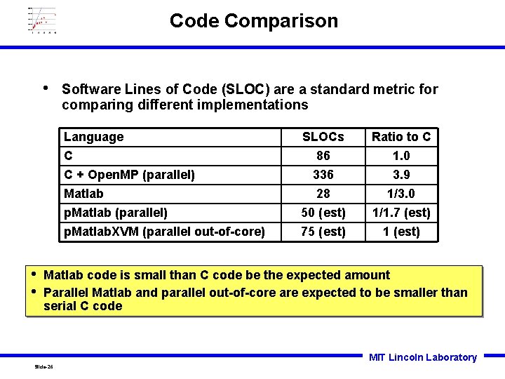
Code Comparison • • • Software Lines of Code (SLOC) are a standard metric for comparing different implementations Language C C + Open. MP (parallel) Matlab p. Matlab (parallel) SLOCs 86 336 28 50 (est) Ratio to C 1. 0 3. 9 1/3. 0 1/1. 7 (est) p. Matlab. XVM (parallel out-of-core) 75 (est) 1 (est) Matlab code is small than C code be the expected amount Parallel Matlab and parallel out-of-core are expected to be smaller than serial C code MIT Lincoln Laboratory Slide-26

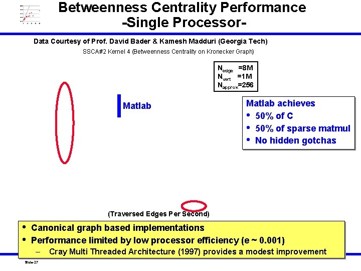
Betweenness Centrality Performance -Single Processor. Data Courtesy of Prof. David Bader & Kamesh Madduri (Georgia Tech) SSCA#2 Kernel 4 (Betweenness Centrality on Kronecker Graph) Nedge =8 M Nvert =1 M Napprox=256 Matlab achieves • 50% of C • 50% of sparse matmul • No hidden gotchas (Traversed Edges Per Second) • • Canonical graph based implementations Performance limited by low processor efficiency (e ~ 0. 001) – Slide-27 Cray Multi Threaded Architecture (1997) provides a modest MIT improvement Lincoln Laboratory

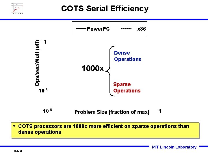
COTS Serial Efficiency Ops/sec/Watt (eff) Power. PC 1 Dense Operations 1000 x 10 -3 10 -6 • x 86 Sparse Operations Problem Size (fraction of max) 1 COTS processors are 1000 x more efficient on sparse operations than dense operations MIT Lincoln Laboratory Slide-28

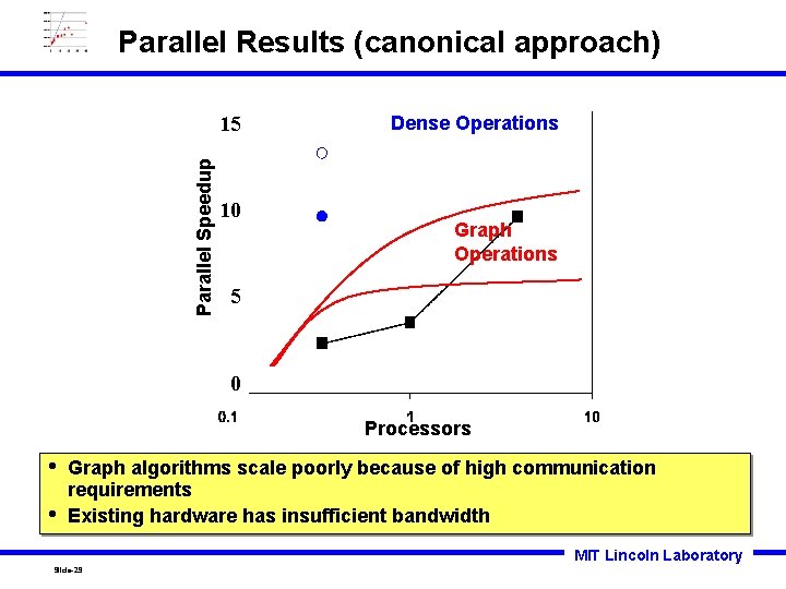
Parallel Results (canonical approach) Parallel Speedup 15 10 Dense Operations Graph Operations 5 0 Processors • • Graph algorithms scale poorly because of high communication requirements Existing hardware has insufficient bandwidth MIT Lincoln Laboratory Slide-29

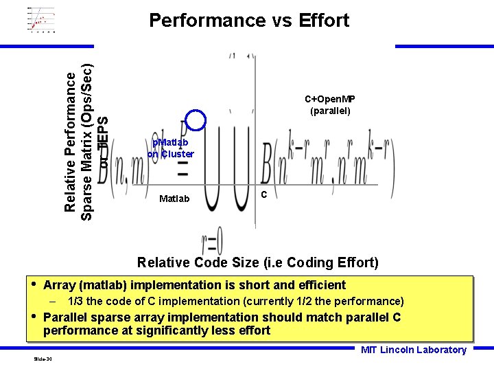
Relative Performance Sparse Matrix (Ops/Sec) or TEPS Performance vs Effort C+Open. MP (parallel) p. Matlab on Cluster Matlab C Relative Code Size (i. e Coding Effort) • Array (matlab) implementation is short and efficient – • 1/3 the code of C implementation (currently 1/2 the performance) Parallel sparse array implementation should match parallel C performance at significantly less effort MIT Lincoln Laboratory Slide-30

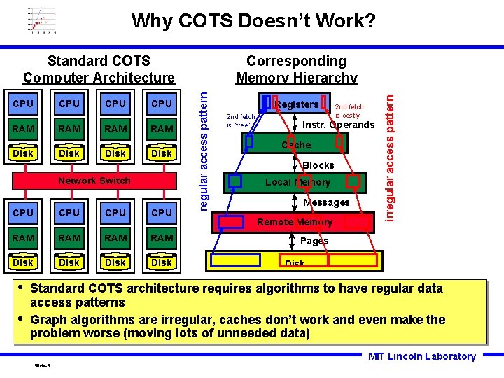
Why COTS Doesn’t Work? CPU RAM Disk Network Switch CPU CPU RAM RAM Disk • • Registers 2 nd fetch is “free” 2 nd fetch is costly Instr. Operands Cache Blocks Local Memory Messages Remote Memory irregular access pattern CPU Corresponding Memory Hierarchy regular access pattern Standard COTS Computer Architecture Pages Disk Standard COTS architecture requires algorithms to have regular data access patterns Graph algorithms are irregular, caches don’t work and even make the problem worse (moving lots of unneeded data) MIT Lincoln Laboratory Slide-31

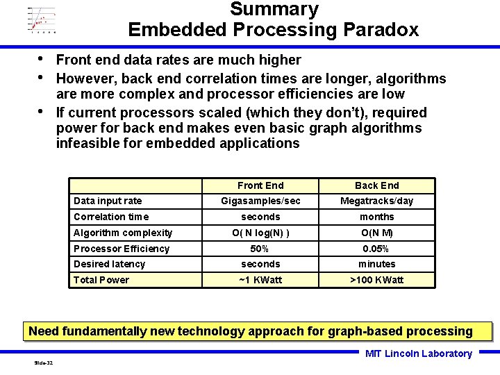
Summary Embedded Processing Paradox • • • Front end data rates are much higher However, back end correlation times are longer, algorithms are more complex and processor efficiencies are low If current processors scaled (which they don’t), required power for back end makes even basic graph algorithms infeasible for embedded applications Front End Back End Gigasamples/sec Megatracks/day seconds months Algorithm complexity O( N log(N) ) O(N M) Processor Efficiency 50% 0. 05% Desired latency seconds minutes Total Power ~1 KWatt >100 KWatt Data input rate Correlation time Need fundamentally new technology approach for graph-based processing MIT Lincoln Laboratory Slide-32

Backup Slides MIT Lincoln Laboratory Slide-33

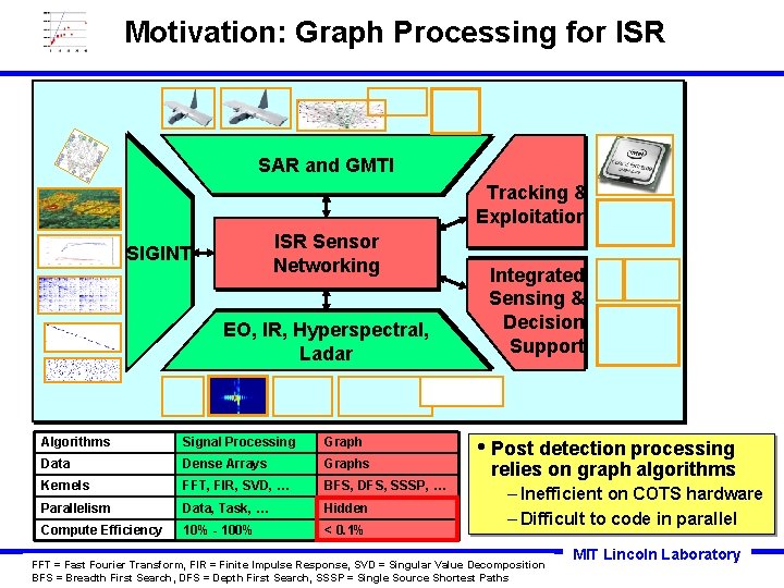
Motivation: Graph Processing for ISR SAR and GMTI Tracking & Exploitation ISR Sensor Networking SIGINT EO, IR, Hyperspectral, Ladar Algorithms Signal Processing Graph Data Dense Arrays Graphs Kernels FFT, FIR, SVD, … BFS, DFS, SSSP, … Parallelism Data, Task, … Hidden Compute Efficiency 10% - 100% < 0. 1% Integrated Sensing & Decision Support • Post detection processing relies on graph algorithms – Inefficient on COTS hardware – Difficult to code in parallel FFT Slide-34 = Fast Fourier Transform, FIR = Finite Impulse Response, SVD = Singular Value Decomposition BFS = Breadth First Search, DFS = Depth First Search, SSSP = Single Source Shortest Paths MIT Lincoln Laboratory