Ligand Screens RAW and B cells Madhu Natarajan

Ligand Screens: RAW and B cells Madhu Natarajan, Rama Ranganathan AFCS Annual Meeting 2004

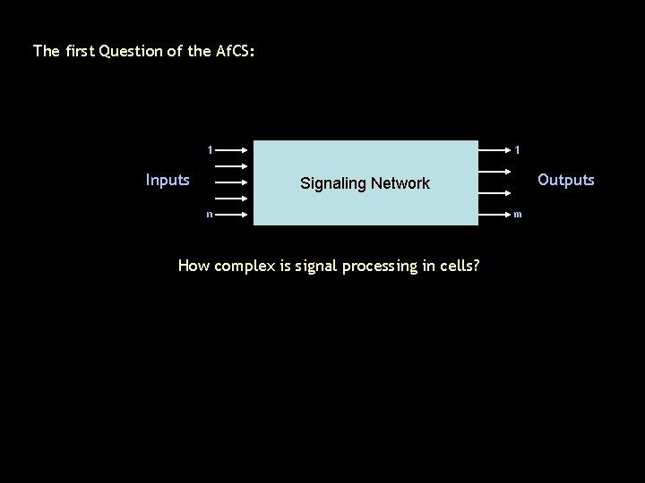
The first Question of the Af. CS: 1 Inputs 1 Outputs Signaling Network n How complex is signal processing in cells? m

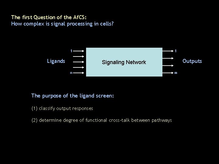
The first Question of the Af. CS: How complex is signal processing in cells? 1 Ligands 1 Outputs Signaling Network n The purpose of the ligand screen: (1) classify output responses (2) determine degree of functional cross-talk between pathways m

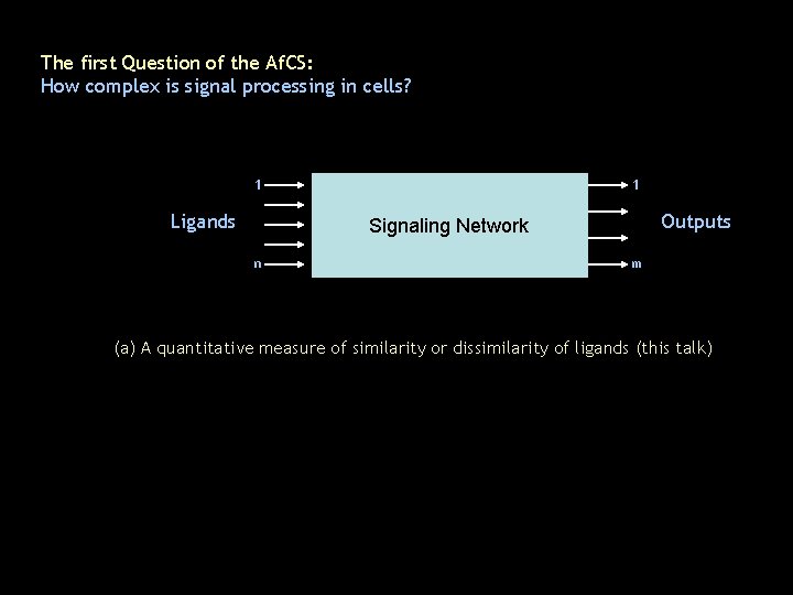
The first Question of the Af. CS: How complex is signal processing in cells? 1 Ligands 1 Outputs Signaling Network n m (a) A quantitative measure of similarity or dissimilarity of ligands (this talk)

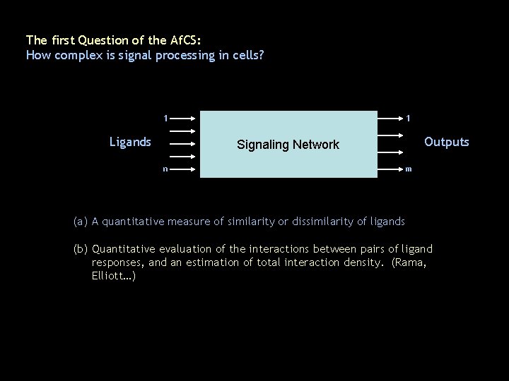
The first Question of the Af. CS: How complex is signal processing in cells? 1 Ligands 1 Outputs Signaling Network n m (a) A quantitative measure of similarity or dissimilarity of ligands (b) Quantitative evaluation of the interactions between pairs of ligand responses, and an estimation of total interaction density. (Rama, Elliott…)

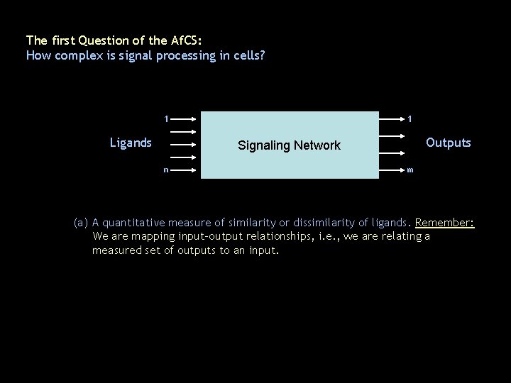
The first Question of the Af. CS: How complex is signal processing in cells? 1 Ligands 1 Outputs Signaling Network n m (a) A quantitative measure of similarity or dissimilarity of ligands. Remember: We are mapping input-output relationships, i. e. , we are relating a measured set of outputs to an input.

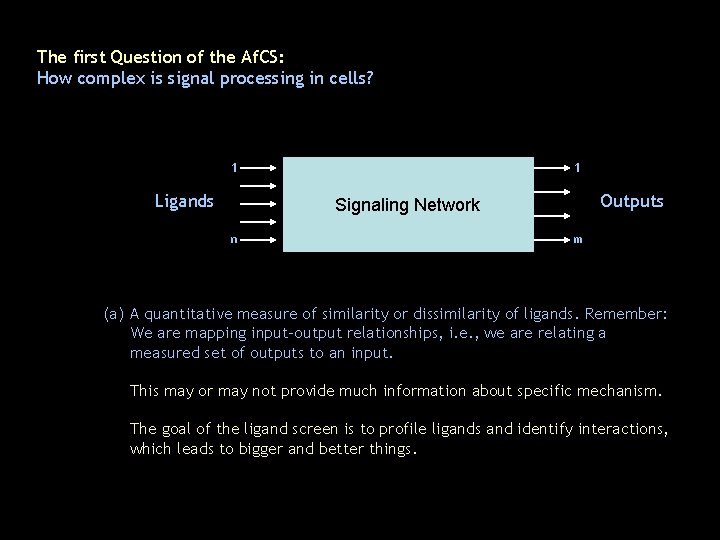
The first Question of the Af. CS: How complex is signal processing in cells? 1 Ligands 1 Outputs Signaling Network n m (a) A quantitative measure of similarity or dissimilarity of ligands. Remember: We are mapping input-output relationships, i. e. , we are relating a measured set of outputs to an input. This may or may not provide much information about specific mechanism. The goal of the ligand screen is to profile ligands and identify interactions, which leads to bigger and better things.

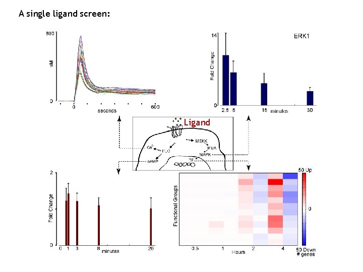
A single ligand screen: Ligand

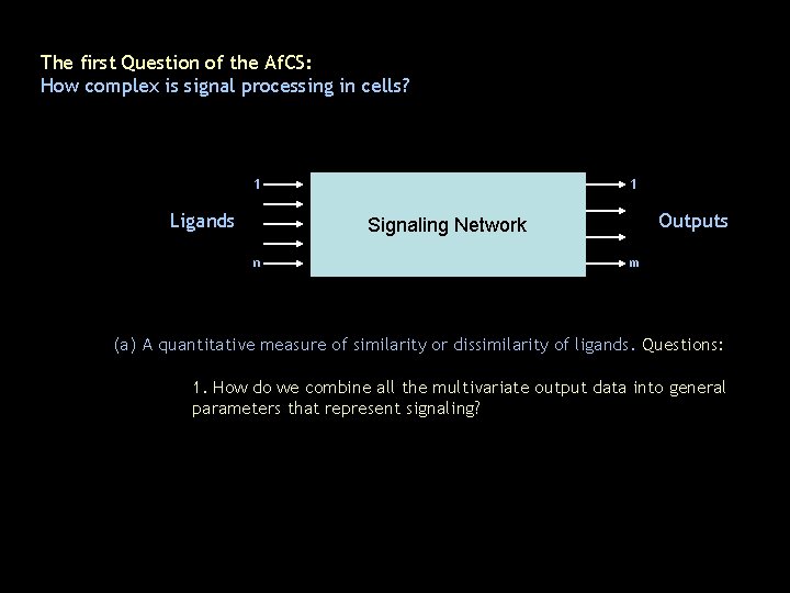
The first Question of the Af. CS: How complex is signal processing in cells? 1 Ligands 1 Outputs Signaling Network n m (a) A quantitative measure of similarity or dissimilarity of ligands. Questions: 1. How do we combine all the multivariate output data into general parameters that represent signaling?

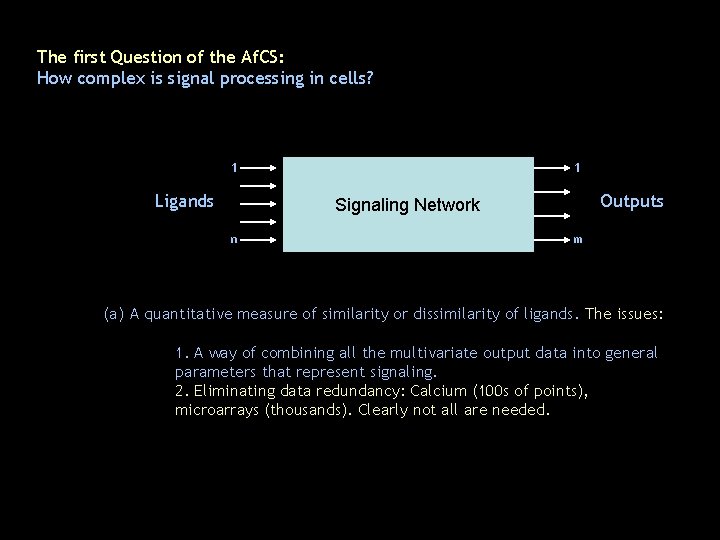
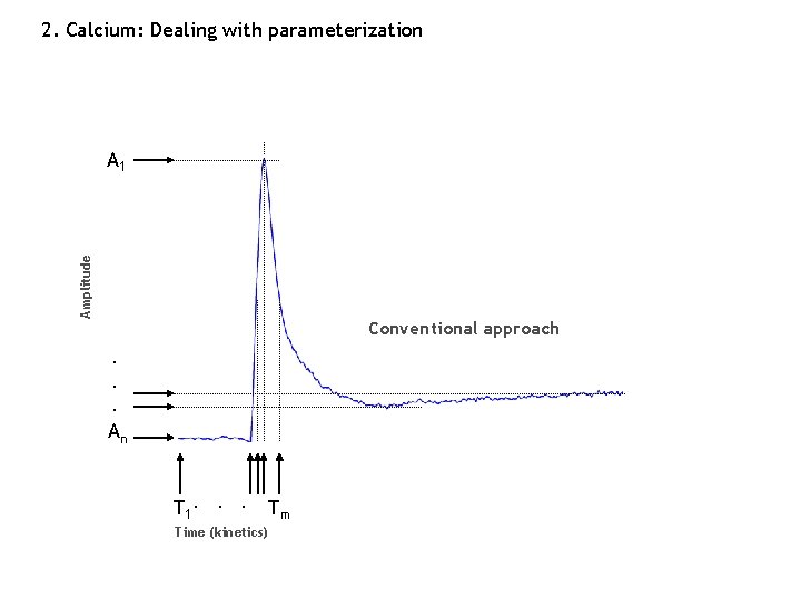
The first Question of the Af. CS: How complex is signal processing in cells? 1 Ligands 1 Outputs Signaling Network n m (a) A quantitative measure of similarity or dissimilarity of ligands. The issues: 1. A way of combining all the multivariate output data into general parameters that represent signaling. 2. Eliminating data redundancy: Calcium (100 s of points), microarrays (thousands). Clearly not all are needed.

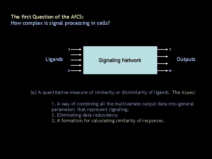
The first Question of the Af. CS: How complex is signal processing in cells? 1 Ligands 1 Outputs Signaling Network n m (a) A quantitative measure of similarity or dissimilarity of ligands. The issues: 1. A way of combining all the multivariate output data into general parameters that represent signaling. 2. Eliminating data redundancy 3. A formalism for calculating similarity of responses.

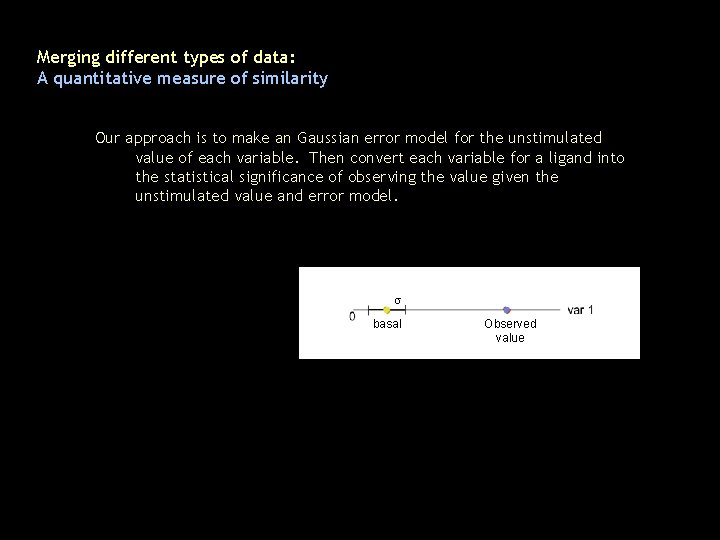
Merging different types of data: A quantitative measure of similarity Our approach is to make an Gaussian error model for the unstimulated value of each variable. Then convert each variable for a ligand into the statistical significance of observing the value given the unstimulated value and error model. s basal Observed value

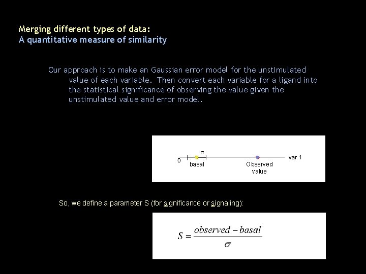
Merging different types of data: A quantitative measure of similarity Our approach is to make an Gaussian error model for the unstimulated value of each variable. Then convert each variable for a ligand into the statistical significance of observing the value given the unstimulated value and error model. s basal So, we define a parameter S (for significance or signaling): Observed value

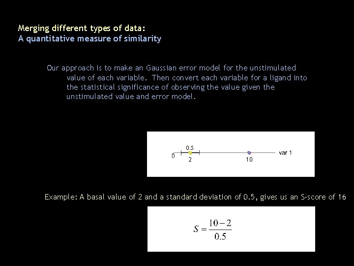
Merging different types of data: A quantitative measure of similarity Our approach is to make an Gaussian error model for the unstimulated value of each variable. Then convert each variable for a ligand into the statistical significance of observing the value given the unstimulated value and error model. 0. 5 2 10 Example: A basal value of 2 and a standard deviation of 0. 5, gives us an S-score of 16

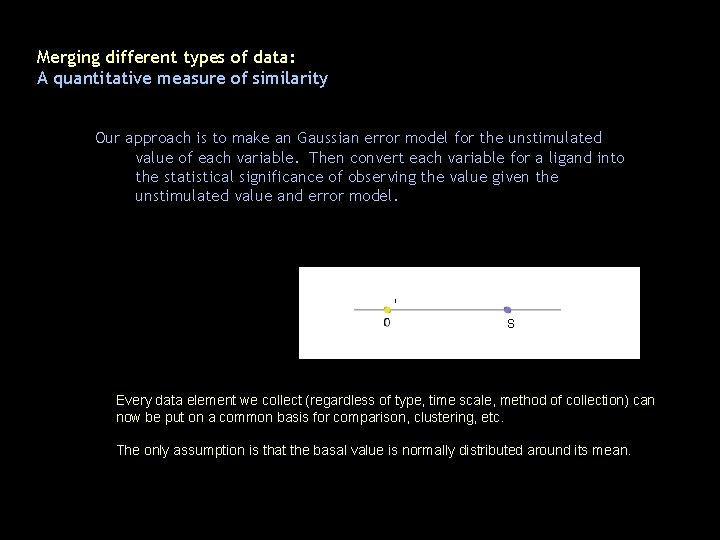
Merging different types of data: A quantitative measure of similarity Our approach is to make an Gaussian error model for the unstimulated value of each variable. Then convert each variable for a ligand into the statistical significance of observing the value given the unstimulated value and error model. s basal S Every data element we collect (regardless of type, time scale, method of collection) can now be put on a common basis for comparison, clustering, etc. The only assumption is that the basal value is normally distributed around its mean.

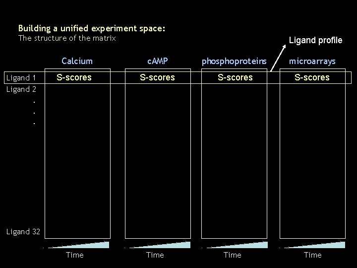
Building a unified experiment space: The structure of the matrix Calcium Ligand 1 Ligand 2 Ligand profile c. AMP phosphoproteins microarrays S-scores Time . . . Ligand 32 Time

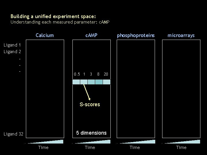
Building a unified experiment space: Understanding each measured parameter: c. AMP Calcium c. AMP phosphoproteins microarrays Time Ligand 1 Ligand 2 . . . 0. 5 1 3 8 20 S-scores 5 dimensions Ligand 32 Time

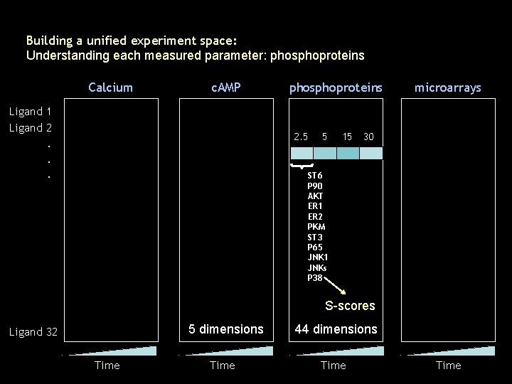
Building a unified experiment space: Understanding each measured parameter: phosphoproteins Calcium c. AMP Ligand 1 Ligand 2 phosphoproteins 2. 5 . . . 5 15 microarrays 30 ST 6 P 90 AKT ER 1 ER 2 PKM ST 3 P 65 JNK 1 JNKs P 38 S-scores 5 dimensions Ligand 32 Time 44 dimensions Time

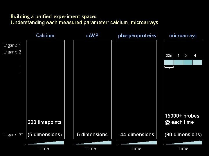
Building a unified experiment space: Understanding each measured parameter: calcium, microarrays Calcium c. AMP phosphoproteins Ligand 1 Ligand 2 microarrays 30 m 1 . . . Time 4 15000+ probes @ each time 200 timepoints Ligand 32 (5 dimensions) 2 5 dimensions Time 44 dimensions (80 dimensions) Time

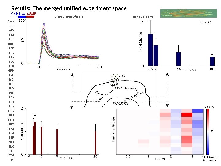
Results: The merged unified experiment space Calcium c. AMP 2 MA 40 L AIG BAF BLC BOM CGS CPG DIM ELC FML GRH IL 4 I 10 IFB IFG IGF LB 4 LPA LPS M 3 A NEB NGF NPY PAF PGE S 1 P SDF SLC TER TGF TNF phosphoproteins microarrays

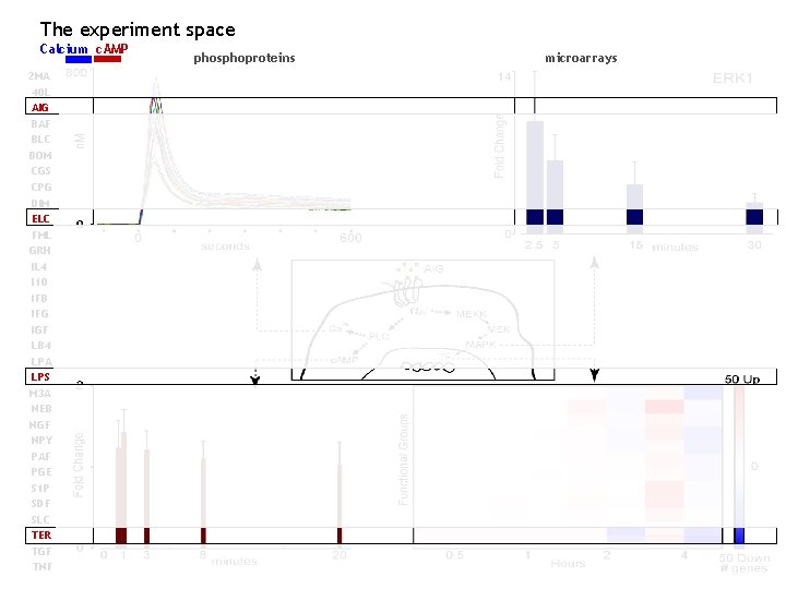
The experiment space Calcium c. AMP 2 MA 40 L AIG BAF BLC BOM CGS CPG DIM ELC FML GRH IL 4 I 10 IFB IFG IGF LB 4 LPA LPS M 3 A NEB NGF NPY PAF PGE S 1 P SDF SLC TER TGF TNF phosphoproteins microarrays

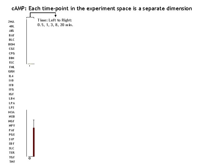
c. AMP: Each time-point in the experiment space is a separate dimension 2 MA 40 L AIG BAF BLC BOM CGS CPG DIM ELC FML GRH IL 4 I 10 IFB IFG IGF LB 4 LPA LPS M 3 A NEB NGF NPY PAF PGE S 1 P SDF SLC TER TGF TNF Time: Left to Right: 0. 5, 1, 3, 8, 20 min.

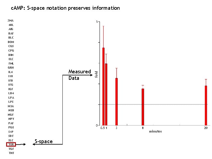
2 MA 40 L AIG BAF BLC BOM CGS CPG DIM ELC FML GRH IL 4 I 10 IFB IFG IGF LB 4 LPA LPS M 3 A NEB NGF NPY PAF PGE S 1 P SDF SLC TER TGF TNF Measured Data fold c. AMP: S-space notation preserves information minutes S-space

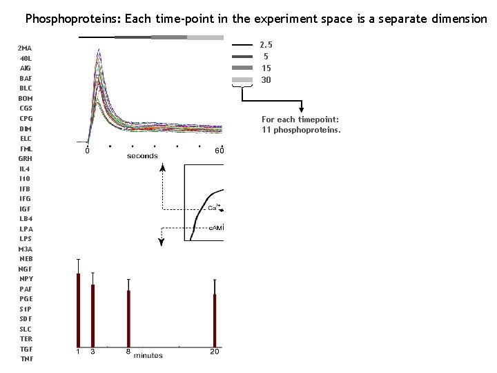
Phosphoproteins: Each time-point in the experiment space is a separate dimension 2 MA 40 L AIG BAF BLC BOM CGS CPG DIM ELC FML GRH IL 4 I 10 IFB IFG IGF LB 4 LPA LPS M 3 A NEB NGF NPY PAF PGE S 1 P SDF SLC TER TGF TNF 2. 5 5 15 30 For each timepoint: 11 phosphoproteins.

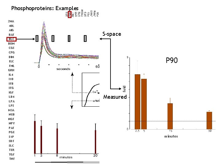
Phosphoproteins: Examples S-space fold 2 MA 40 L AIG BAF BLC BOM CGS CPG DIM ELC FML GRH IL 4 I 10 IFB IFG IGF LB 4 LPA LPS M 3 A NEB NGF NPY PAF PGE S 1 P SDF SLC TER TGF TNF Measured minutes

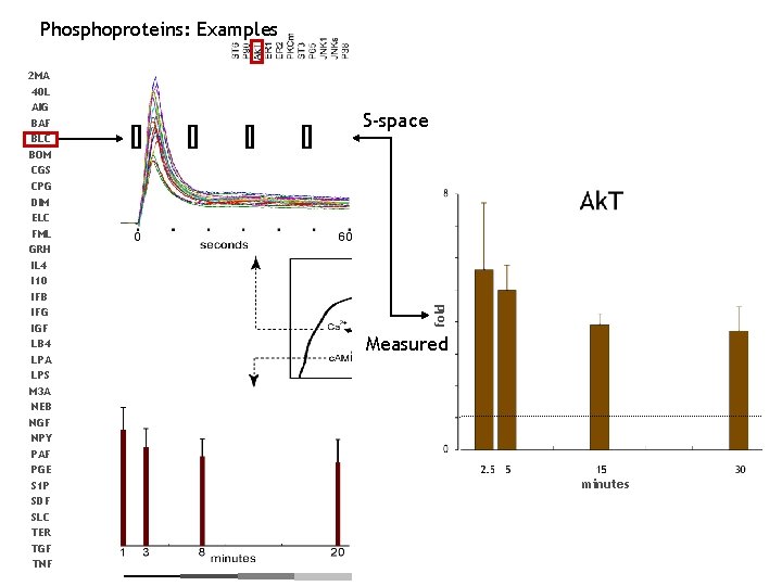
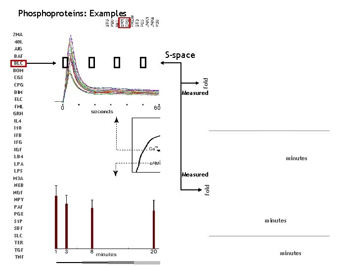
Phosphoproteins: Examples fold S-space Measured minutes Measured fold 2 MA 40 L AIG BAF BLC BOM CGS CPG DIM ELC FML GRH IL 4 I 10 IFB IFG IGF LB 4 LPA LPS M 3 A NEB NGF NPY PAF PGE S 1 P SDF SLC TER TGF TNF minutes

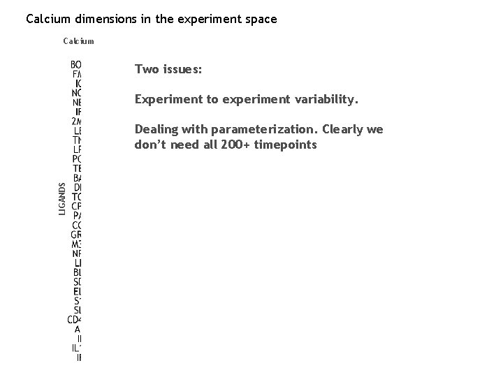
Calcium dimensions in the experiment space Calcium Two issues: Experiment to experiment variability. LIGANDS Dealing with parameterization. Clearly we don’t need all 200+ timepoints

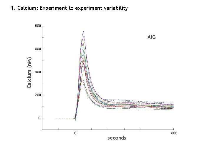
1. Calcium: Experiment to experiment variability Calcium (n. M) AIG seconds

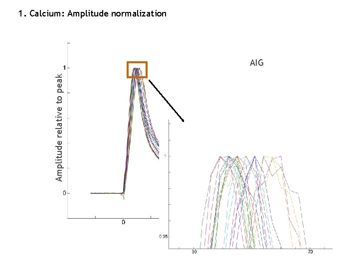
1. Calcium: Amplitude normalization Amplitude relative to peak AIG seconds

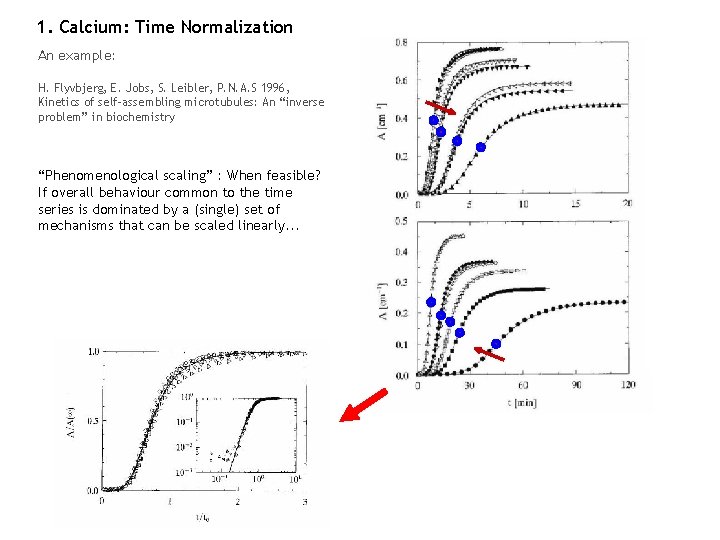
1. Calcium: Time Normalization An example: H. Flyvbjerg, E. Jobs, S. Leibler, P. N. A. S 1996, Kinetics of self-assembling microtubules: An “inverse problem” in biochemistry “Phenomenological scaling” : When feasible? If overall behaviour common to the time series is dominated by a (single) set of mechanisms that can be scaled linearly. . . Madhu Natarajan: May 04, 2004

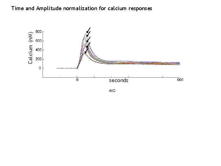
Calcium (n. M) Time and Amplitude normalization for calcium responses seconds T 10 T

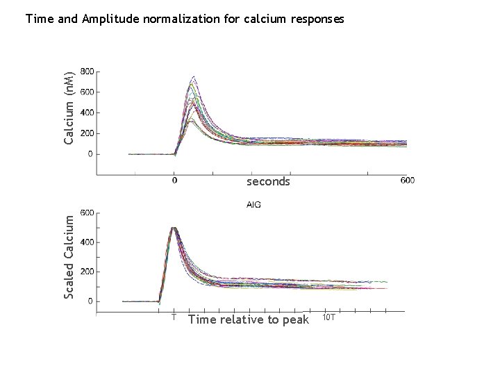
Calcium (n. M) Time and Amplitude normalization for calcium responses Scaled Calcium seconds T Time relative to peak 10 T

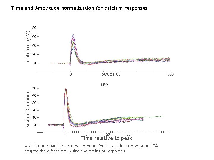
Calcium (n. M) Time and Amplitude normalization for calcium responses Scaled Calcium seconds T 10 T 20 T 30 T Time relative to peak A similar mechanistic process accounts for the calcium response to LPA despite the difference in size and timing of responses

Scaled Calcium Scaling on the time-axis does not reduce discrimination between ligands T 10 T 20 T 30 T Time relative to LPA peak The results are not artefactual despite the similarity of calcium profiles

1. Calcium day-to-day response differences are not “biological” Experiments on 7 different days

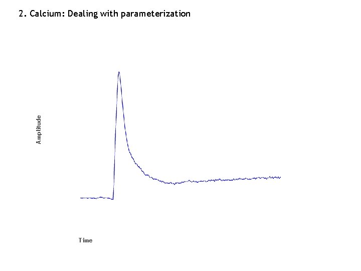
Amplitude 2. Calcium: Dealing with parameterization Time

2. Calcium: Dealing with parameterization Amplitude A 1 Conventional approach . . . An . . . T 1 Tm Time (kinetics)

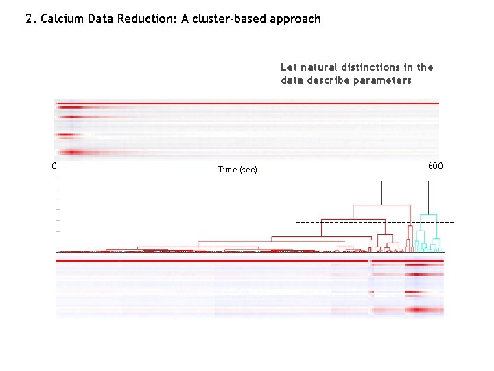
2. Calcium Data Reduction: A cluster-based approach Let natural distinctions in the data describe parameters 0 Time (sec) 600

2. Calcium Data Reduction Data separation mirrors what we have intuitively been using all along

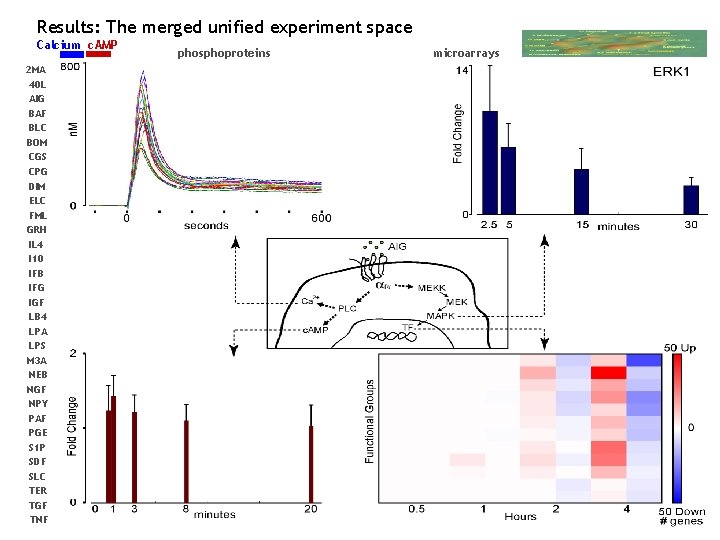
Results: The merged unified experiment space Calcium c. AMP 2 MA 40 L AIG BAF BLC BOM CGS CPG DIM ELC FML GRH IL 4 I 10 IFB IFG IGF LB 4 LPA LPS M 3 A NEB NGF NPY PAF PGE S 1 P SDF SLC TER TGF TNF phosphoproteins microarrays

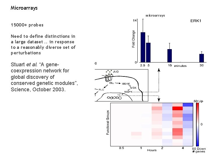
Microarrays microarrays 15000+ probes Need to define distinctions in a large dataset. . in response to a reasonably diverse set of perturbations Stuart et al. “A genecoexpression network for global discovery of conserved genetic modules”, Science, October 2003.

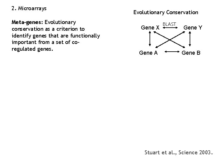
2. Microarrays Meta-genes: Evolutionary conservation as a criterion to identify genes that are functionally important from a set of coregulated genes. Evolutionary Conservation Gene X Gene A BLAST Gene Y Gene B Stuart et al. , Science 2003.

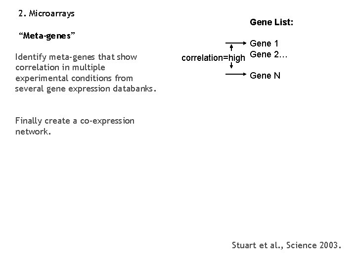
2. Microarrays “Meta-genes” Identify meta-genes that show correlation in multiple experimental conditions from several gene expression databanks. Gene List: Gene 1 correlation=high Gene 2… Gene N Finally create a co-expression network. Stuart et al. , Science 2003.

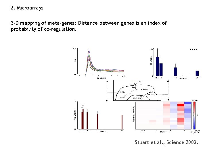
2. Microarrays 3 -D mapping of meta-genes: Distance between genes is an index of probability of co-regulation. Stuart et al. , Science 2003.

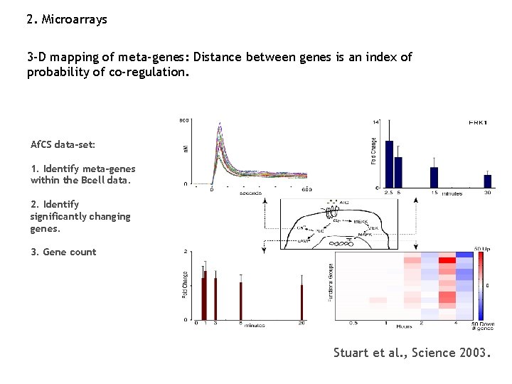
2. Microarrays 3 -D mapping of meta-genes: Distance between genes is an index of probability of co-regulation. Af. CS data-set: 1. Identify meta-genes within the Bcell data. 2. Identify significantly changing genes. 3. Gene count Stuart et al. , Science 2003.

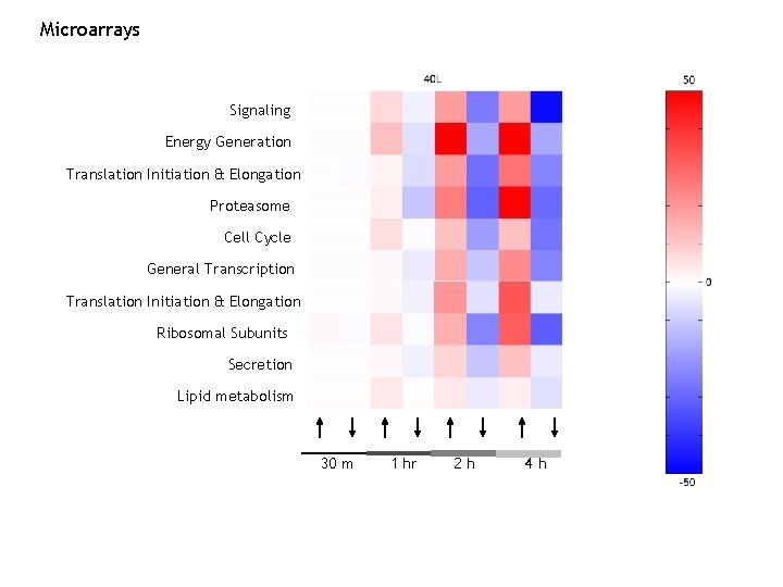
Microarrays Signaling Energy Generation Translation Initiation & Elongation Proteasome Cell Cycle General Transcription Translation Initiation & Elongation Ribosomal Subunits Secretion Lipid metabolism 30 m 1 hr 2 h 4 h

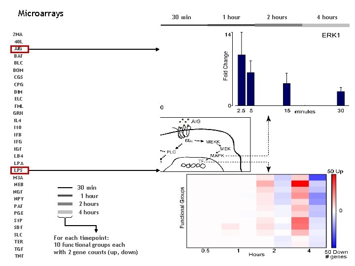
Microarrays 2 MA 40 L AIG BAF BLC BOM CGS CPG DIM ELC FML GRH IL 4 I 10 IFB IFG IGF LB 4 LPA LPS M 3 A NEB NGF NPY PAF PGE S 1 P SDF SLC TER TGF TNF 30 min 1 hour 2 hours 4 hours For each timepoint: 10 functional groups each with 2 gene counts (up, down) 1 hour 2 hours 4 hours

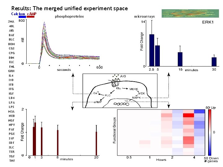
Results: The merged unified experiment space Calcium c. AMP 2 MA 40 L AIG BAF BLC BOM CGS CPG DIM ELC FML GRH IL 4 I 10 IFB IFG IGF LB 4 LPA LPS M 3 A NEB NGF NPY PAF PGE S 1 P SDF SLC TER TGF TNF phosphoproteins microarrays

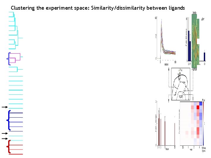
Clustering the experiment space: Similarity/dissimilarity between ligands 20 -20

Summary: 1. A simple transformation of raw data variables into dimensionless S variables (units of significance) permits construction of an unified experiment space of all data, regardless of source or differences in intrinsic dynamic range and signal to noise.

Summary: 1. A simple transformation of raw data variables into dimensionless S variables (units of significance) permits construction of an unified experiment space of all data, regardless of source or differences in intrinsic dynamic range and signal to noise. 2. A potentially serious danger is over-parameterization, the usage of many non-independent variables to represent a biological process (say, the inactivation of a calcium response). We have shown two ways to address this problem on the calcium and microarray dimensions.

Summary: 1. A simple transformation of raw data variables into dimensionless S variables (units of significance) permits construction of an unified experiment space of all data, regardless of source or differences in intrinsic dynamic range and signal to noise. 2. A potentially serious danger is over-parameterization, the usage of many non-independent variables to represent a biological process (say, the inactivation of a calcium response). We have shown two ways to address this problem on the calcium and microarray dimensions. 3. We have assembled an experiment space of 32 ligands by 134 parameters that represents the single ligand profiles for each ligand. This space can be clustered to identify similarities/dissimilarities between ligands.

Summary: 1. A simple transformation of raw data variables into dimensionless S variables (units of significance) permits construction of an unified experiment space of all data, regardless of source or differences in intrinsic dynamic range and signal to noise. 2. A potentially serious danger is over-parameterization, the usage of many non-independent variables to represent a biological process (say, the inactivation of a calcium response). We have shown two ways to address this problem on the calcium and microarray dimensions. 3. We have assembled an experiment space of 32 ligands by 134 parameters that represents the single ligand profiles for each ligand. This space can be clustered to identify similarities/dissimilarities between ligands. 4. The method of analysis is independent of cell type or assays within the ligand screen. It is equally applicable to the B cell or the RAW cell data.

Summary: 1. A simple transformation of raw data variables into dimensionless S variables (units of significance) permits construction of an unified experiment space of all data, regardless of source or differences in intrinsic dynamic range and signal to noise. 2. A potentially serious danger is over-parameterization, the usage of many non-independent variables to represent a biological process (say, the inactivation of a calcium response). We have shown two ways to address this problem on the calcium and microarray dimensions. 3. We have assembled an experiment space of 32 ligands by 134 parameters that represents the single ligand profiles for each ligand. This space can be clustered to identify similarities/dissimilarities between ligands. 4. The method of analysis is independent of cell type or assays within the ligand screen. It is equally applicable to the B cell or the RAW cell data. Looking ahead: Applicability to the double ligand screen and beyond: Rama, Elliott.

Acknowledgements Rama Ranganathan Paul Sternweis Elliott Ross Ron Taussig Mel Simon Al Gilman