Leverage and Asymmetric Volatility The Firm Level Evidence

Leverage and Asymmetric Volatility: The Firm Level Evidence Presented by Stefano Mazzotta Kennesaw State University joint work with Jan Ericsson, Mc. Gill University and Xiao Huang, Kennesaw State University

Outline n n n Introduction Asymmetric volatility and leverage The panel data model Time varying risk premium and leverage Empirical results Conclusion

Two explanations of asymmetric volatility: n Leverage effect (e. g. Black (1976) Christie (1982)): q n Stock price↓⇒Leverage↑⇒Risk↑⇒Volatility↑ Time varying risk premium, (e. g. French et al. (1987) Campbell and Hentschel (1992), Bekaert and Wu (2000) q Persistent volatility↑⇒Required rate of return↑⇒Stock price↓

Leverage and volatility n The traditional leverage effect argument states that as stock prices drop, increased leverage pushes up the equity volatility for a given asset volatility (business risk). n This is the spirit of the test in Christie (1982). But from a firm’s perspective, the choice of leverage and volatility is a joint one, at least in the medium to long term. Leverage will depend on volatility and vice versa. Thus a two way relationship needs to be modeled n

Traditional capital structure revisited n The tradeoff theory of capital structure is taught in all introductory finance texts but is often viewed with skepticism by researchers as a means of explaining capital structure empirically. q Recent work provides a more rosy view of the canonical ideas and question existing empirical work n Molina (2005, JF) highlights the impact of neglecting endogeneity when assessing empirically the validity of the tradeoff theory.

The leverage effect revisited n n This skepticism has also extended to the literal interpretation of the leverage effect. We ask what can be learnt q q q By reconsidering the leverage effect at the individual firm level in the presence of an alternative explanation (time varying risk premia) By allowing leverage and volatility to influence each other in a two way system Captures also long term effects.

Our contributions n n A panel vector autoregression (PVAR) approach to study the dynamics of leverage, volatility and risk premium jointly Control firm level heterogeneity We find leverage effect is more important than volatility feedback effect and it accumulates over the time Volatility feedback exists but does not reinforce over the time.

The data n n n n CRSP quarterly database COMPUSTAT daily database merged using the identifiers CUSIP, and CNUM. Sample period: 1971 2005. 116, 861 firm quarter observations The debt is computed as the sum of total liabilities (data 54) and preferred stock (data 55). Equity is computed as the product of common shares outstanding (data 61) and price at the end of the quarter (data 14). The leverage variable QRit is the ratio of debt over equity at time t for firm i. Quartiles are obtained based on the average QRit. We consider firms with QR>100 outliers and eliminate them.

Empirics Leverage: QRit = Debt / Equity for ¯rm iat t ime t Realized volat ility: ¾it = Risk premium: r ¹ it = PQ h= PQ 1 h= 1 rm ; t¡ r 2 q P 1 ; h m ; t¡ 1 ; h P Q r 2 h= 1 ith Q [r r t¡ 1; h] h m; t¡ 1; h= 1 i; where Q = rit = rmt = number of days in each quart er ret urn of st ock iin excess of T Bill market ret urn in excess of T Bill

Stats: QR M ean M edian M aximum M inimum St d. Dev. Skewness K urt osis Jarque Bera Probability Observat ions Q 1 0. 184 0. 130 4. 264 0. 000 0. 192 3. 912 39. 669 1427190 0 24365 Panel 1: All Sample Q 2 Q 3 0. 540 1. 315 0. 431 1. 095 8. 882 39. 678 0. 000 0. 001 0. 477 1. 091 3. 546 4. 715 29. 989 79. 637 1025705 7964801 0 0 31613 32061 Q 4 6. 984 2. 448 26377. 000 0. 003 235. 211 99. 435 10342. 310 1. 34 E+ 11 0 30018 A ll 2. 315 0. 708 26377. 000 0. 000 118. 637 197. 145 40659. 870 8. 13 E+ 12 0 118057 Q 1 0. 182 0. 129 4. 264 0. 000 0. 190 3. 812 38. 352 1311161 0 24060 Panel 2: No Out liers Q 2 Q 3 0. 533 1. 288 0. 425 1. 066 8. 882 39. 678 0. 000 0. 001 0. 473 1. 089 3. 599 4. 829 30. 871 81. 692 1082949 8279855 0 0 31367 31614 Q 4 3. 739 2. 395 98. 387 0. 003 5. 284 6. 779 74. 022 6. 50 E+ 06 0 29820 A ll 1. 483 0. 698 98. 387 0. 000 3. 068 10. 633 195. 074 1. 82 E+ 08 0 116861

Stats: Realized Volatility Mean Median Maximum Minimum St d. Dev. Skewness Kurt osis Jarque Bera Probability Observat ions Q 1 0. 594 0. 515 10. 360 0. 000 0. 375 3. 332 39. 915 1410678 0 24060 No Out liers Q 2 Q 3 0. 574 0. 521 0. 481 0. 425 7. 399 6. 728 0. 000 0. 380 0. 409 2. 794 3. 112 23. 590 23. 750 594877. 4 618184. 5 0 0 31367 31614 Q 4 0. 488 0. 352 7. 893 0. 000 0. 450 3. 382 25. 274 6. 73 E+ 05 0 29820 All 0. 542 0. 447 10. 360 0. 000 0. 408 3. 105 26. 442 2. 86 E+ 06 0 116861

Stats: CAPM required returns Mean Median Maximum Minimum St d. Dev. Skewness K urt osis Jarque Bera Probability Observat ions Q 1 0. 036 0. 016 5. 420 3. 544 0. 381 0. 471 11. 513 73534. 3 0 24060 No Out liers Q 2 Q 3 0. 032 0. 024 0. 013 0. 011 7. 859 7. 623 3. 057 4. 630 0. 346 0. 312 0. 109 0. 136 19. 347 25. 290 349308. 4 654536. 4 0 0 31367 31614 Q 4 0. 020 0. 009 4. 332 4. 697 0. 280 0. 365 22. 351 465905. 9 0 29820 All 0. 028 0. 012 7. 859 4. 697 0. 329 0. 260 19. 081 1260513 0 116861

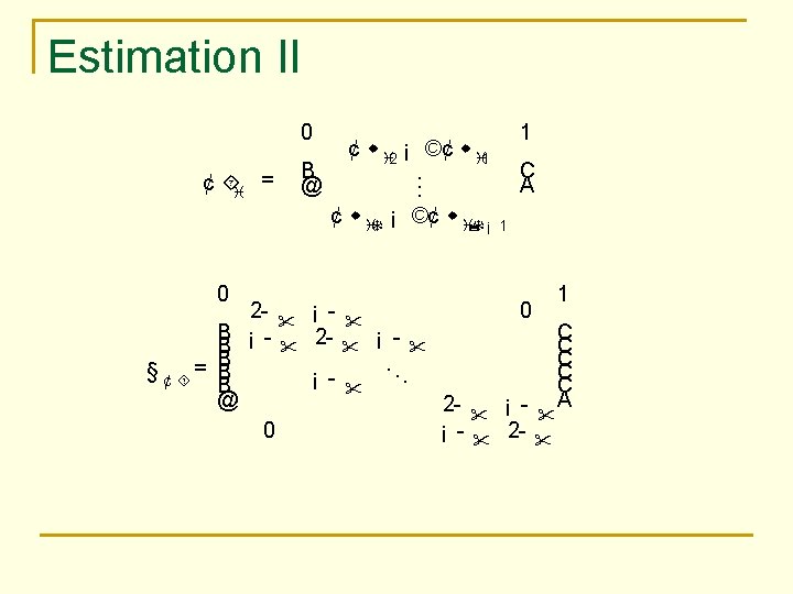
The PVAR model w it = ®i+ ©w i; t¡ 0 1 1 + " it 0 QRit Á11 ®i 1 w it = @ ¾it A ; ®i = @ ®i 2 A ; © = @ Á21 Á31 r ®i 3 ¹ it Á12 Á22 Á32 1 Á13 Á23 A Á33 0 ¾"11 i: i: d: v " (0; ") and "= @ ¾"21 i; t ¾"31 i= 1; ¢¢¢ ; N and t= 1; ¢¢¢ ; T: 1 ¾"22 ¾"32 A ¾"11

Pesaran’s QMLE Estimation Take ¯rst di®erences ¢ w it = ©¢ w i; t¡ 1 + ¢" it T he log likelihood funct ion is N m. N (T ¡ 1) 1 XN 0§ ¡ 1 ¢ ´ l(µ) = ¡ log (2¼) ¡ log j§ ¢ ´j ¡ ¢ ´i i ¢´ 2 2 2 i= 1 where µ= (Á11 ; Á12 ; Á13 ; Á21 ; Á22 ; Á23 ; Á32 ; Á31 ; Á33 ; !11 ; !21 ; !31 ; !22 ; !33 ) 0 0 1 2 !11 !21 !11 !31 2 + ! 2 !11 !21 !31 + !22 !32 A "= @ !11 !21 22 2 + ! 2 !11 !31 !21 !31 + !22 !32 !11 22 33

Bivariate PVAR ¢ QRi; t = Á11 ¢ QRi; t¡ 1 + Á12 ¢ ¾i; t¡ 1 + ¢ " t 1 i; ¢ ¾i; t = Á21 ¢ QRi; t¡ 1 + Á22 ¢ ¾i; t¡ 1 + ¢ " t 2 i; Á1; 1 Á1; 2 Á2; 1 Á2; 2 !1; 1 !2; 2 Q 1 0. 85 0. 01 0. 13 0. 35 0. 10 0. 02 0. 29 t st at s 51. 54 2. 42 5. 33 8. 92 23. 16 5. 42 27. 30 Q 2 0. 83 0. 04 0. 07 0. 39 0. 27 0. 02 0. 29 Panel t st at s 82. 74 3. 98 8. 86 20. 10 29. 90 6. 36 34. 83 2: No out liers Q 3 t st at s 0. 86 55. 76 0. 14 5. 52 0. 04 11. 82 0. 41 20. 15 0. 64 18. 02 0. 02 7. 34 0. 29 36. 47 Q 4 0. 88 0. 62 0. 01 0. 49 2. 79 0. 04 0. 30 t st at s 36. 48 6. 14 8. 71 16. 34 17. 39 7. 07 29. 57 All 0. 89 0. 21 0. 02 0. 43 1. 46 0. 02 0. 29 t st at s 40. 27 7. 13 11. 47 30. 83 18. 25 9. 22 63. 78

Trivariate PVAR + Á ¢¾ ¢ QR = Á ¢ QR t i; 11 t¡ 1 i; 12 ¢ ¾it = Á21 ¢ QRi; t¡ 1 + Á22 ¢ ¾i; t¡ ¢ ri; t = Á31 ¢ QRi; t¡ 1 + Á32 ¢ ¾i; t¡ Á1; 1 Á1; 2 Á1; 3 Á2; 1 Á2; 2 Á2; 3 Á3; 1 Á3; 2 Á3; 3 !1; 1 !2; 1 !3; 1 !2; 2 !3; 3 Q 1 0. 8459 0. 0083 0. 0085 0. 1291 0. 3543 0. 0411 0. 0002 0. 0038 0. 0370 0. 1036 0. 0164 0. 0068 0. 2932 0. 0088 0. 0955 t st at s 51. 47 2. 35 0. 88 4. 06 9. 01 1. 64 0. 06 1. 46 1. 14 23. 18 3. 11 15. 08 27. 35 18. 40 27. 09 + Á13 ¢ ri; t¡ 1 + ¢ " it 1 + Á23 ¢ ri; t¡ 1 + ¢ " it 2 1 + Á33 ¢ ri; t¡ 1 + ¢ " it 3 1 t¡ 1 i; Trivariat e Panel VA R. No out liers. t st at s Q 2 Q 3 Q 4 0. 8329 80. 65 0. 8601 56. 13 0. 8830 0. 0377 2. 10 0. 1363 4. 77 0. 6157 0. 1229 0. 15 0. 2469 1. 79 1. 1362 0. 0695 8. 70 0. 0442 11. 73 0. 0127 0. 3916 20. 07 0. 4126 20. 12 0. 4931 0. 0571 0. 37 0. 0169 7. 54 0. 0594 0. 0006 0. 27 0. 0013 10. 71 0. 0004 0. 0016 0. 24 0. 0004 1. 20 0. 0052 0. 0346 1. 55 0. 0302 1. 83 0. 0276 0. 2732 29. 66 0. 6349 18. 13 2. 7925 0. 0248 3. 48 0. 0246 6. 82 0. 0395 0. 0076 12. 68 0. 0077 28. 54 0. 0061 0. 2871 34. 90 0. 2916 36. 50 0. 2974 0. 0056 13. 91 0. 0033 16. 37 0. 0039 0. 0865 33. 29 0. 0781 31. 94 0. 0697 t st at s 36. 35 5. 34 0. 63 8. 59 16. 53 0. 16 5. 61 8. 29 5. 29 17. 46 7. 14 27. 78 29. 73 16. 36 30. 14 A ll 0. 8909 0. 2079 0. 2805 0. 0171 0. 4252 0. 0228 0. 0005 0. 0028 0. 0331 1. 4602 0. 0241 0. 0044 0. 2936 0. 0054 0. 0825 t st at s 40. 28 6. 07 3. 63 11. 67 30. 61 1. 36 2. 30 2. 55 11. 75 18. 26 8. 86 9. 43 63. 79 8. 35 95. 45

Main results ^ gives a much larger leverage e®ect compared t o est imat es in previous ² Á 21 research. ^ and Á ^ show leverage e®ect accumulat es. ² Á 21 12 ^ con¯rms volat ility feedback ² Á 32 ^ and Á ^ show volat ility feedback does not accumulat e. ² Á 32 23

Wald Test H o: Á13 ; Á23 ; Á31 ; Á32 ; Á33 are joint ly = 0 Quart ile Wald st at ist ics p val Q 1 342. 155 0. 000 Q 2 295. 482 0. 000 Q 3 41. 270 0. 000 Q 4 326. 315 0. 000 All 908. 035 0. 000

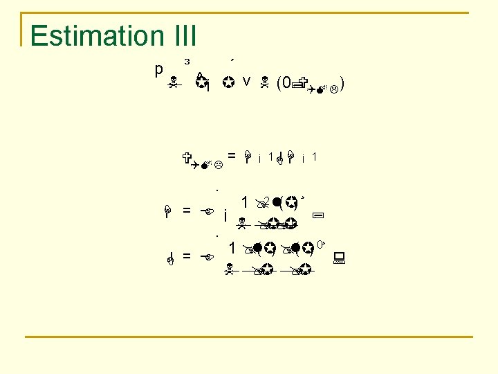
Contemporaneous Correlations ½(QR; ¾) ½(r; ¾) ½(QR; r) Q 1 0. 056 0. 071 0. 096 t st at s 554. 74 788. 15 733. 27 Q 2 0. 086 0. 088 0. 071 t st at s 487. 98 812. 20 251. 86 ½(QR; ¾) ½(r; ¾) ½(QR; r) Q 3 0. 084 0. 098 0. 050 t st at s 605. 24 695. 05 195. 49 Q 4 0. 132 0. 087 0. 066 t st at s 409. 50 508. 72 188. 75 All 0. 082 0. 053 0. 070 t st at s 981. 78 1641. 44 1094. 12

Contemporanous Correlation ² ½(QR; ¾) > 0 ) cont emporaneous leverage e®ect ² ½(¹r; ¾) < 0 ) no cont emporaneous volat ility feedback

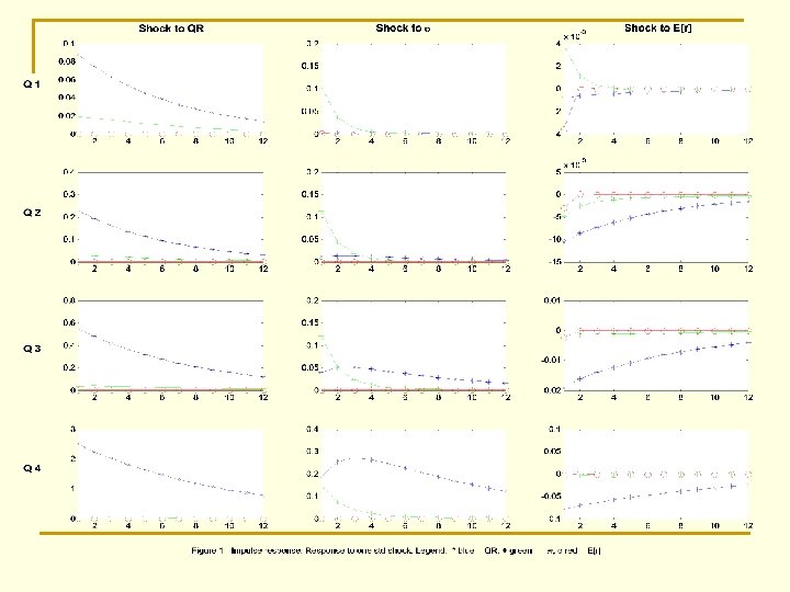
Impulse response function ² A shock from QR a®ect s QR; ¾and r ¹ persist ent ly. ² Volat ility shock a®ect s leverage when leverage rat io is high. ² Shock from required ret urn a®ect s all variables negat ively.

Concluding remarks n n n We reconfirm the relationship between equity volatility and the debt ratio presented in Christie (1982) across the four leverage quartiles. Our main finding is that a dynamic set up is important to capture the cumulative leverage effect. Financial leverage is an economically more significant determinant of equity volatilities than previous work has documented, and its effect accumulates over time. The accumulation of the leverage effect over time renders it at least up to five times larger than previously thought. Our study suggests that past results may be due to not fully allowing for the endogenous nature of the relationship between capital structure and business risk.