Levels of Measurement Levels of Measurement IntervalResponses are

Levels of Measurement

Levels of Measurement • Interval-Responses are measured on a standardized, universal scale (e. g. count, percent, dollars, inches, hours, etc. ). May also include sums, averages, and ratios of ordinal data or ordinal data with more than 7 scale points. • Ordinal-There are more than two options and the options can be ordered (e. g. income brackets, Likert scale, small/medium/large, etc. ) • Binary-There are exactly two options (e. g. yes/no, on/off, male/female). By best practice, these should be coded 0/1 (no/yes). • Categorical-There are more than two options and the options cannot be ordered (e. g. colors, race, etc. ). These must generally be converted to sets of binary variables to be statistically useful. • Nominal-Each individual response is unique and cannot be meaningfully ordered. Typically, the purpose of nominal data is to identify or name the observation (e. g. ID number, name, street address, phone number).

Performance Measurement Techniques

Types of Measures • Performance Measurement: How is our organization or program performing now (ongoing)? • Program Evaluation: One-time study linked to the life cycle of the program. Most common form is outcome evaluation, which occurs retrospectively. However, other types of program evaluation (e. g. needs assessment) may occur prospectively. • Effectiveness measures generally focus on results of a program or treatment. Generally, involves outputs and outcomes. • Efficiency measures generally focus on the cost to produce a good or service, including non-monetary resources. These are generally calculated in ratios of outputs over inputs (outputs/inputs) or outcomes over inputs (outcomes/inputs).

Some Useful Composite Variables • Workload ratios are ratios of activities to inputs. • Benchmarks are standards (internal or external) against which performance is evaluated. These are standards with which performance is compared. • Equity measures are comparisons of outputs or outcomes across groups-equity measures of interest compare data for privileged groups with disadvantaged groups. • Indexes are generally sums or averages of a group of variables that measure the same underlying construct or different dimension of an underlying construct. • Efficiency measures generally focus on the cost to produce a good or service, including non-monetary resources. These are generally calculated in ratios of outputs over inputs (outputs/inputs) or outcomes over inputs (outcomes/inputs).

Measures of Central Tendency

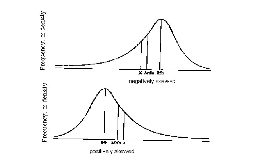
Uses of Measures of Central Tendency • Quickly describe a sample • Identify where the sample is “centered” • Examine skewness • Identify whether or not a dataset appears to be clean • Verify that the values make sense

Central Tendency Questions • In my sample, what is the “center” of the data for this variable? • Mean • Median • In my sample, what is the most common value for this variable? • Mode • How common in my sample is value “x” for this variable? • Proportion • Percent

Measures of Central Tendency

Measures of Dispersion

Uses of Measures of Dispersion • Quickly describe a sample • Identify the full range of observed values • Determine how close together or spread apart values appear to be • Identify whether or not a dataset appears to be clean • Ensure that the highest and lowest values are within expected ranges

Dispersion Questions • In my sample, what are the highest and lowest values for this variable? • Maximum • Minimum • In my sample, how spread out is the data for this variable? • Standard deviation • Interquartile range • Is my data symmetrical? • Skewness • Quantiles

Measures of Dispersion

Frequency Distributions

Age of Math Student 6 M 1 or e 60 59 58 57 56 55 54 53 52 51 50 49 48 47 46 45 44 43 42 41 40 39 38 37 36 35 34 33 32 31 30 29 28 27 26 25 24 23 22 21 20 19 18 Frequency Histogram of Age of SLCC Math Students (n=500) 60 50 40 30 20 10 0

Histogram of Age of SLCC Math Students (n=131, 034) 14000 12000 8000 6000 4000 2000 61 60 59 58 57 56 55 54 53 52 51 50 49 48 Age of Math Student 47 46 45 44 43 42 41 40 39 38 37 36 35 34 33 32 31 30 29 28 27 26 25 24 23 22 21 20 19 0 18 Frequency 10000

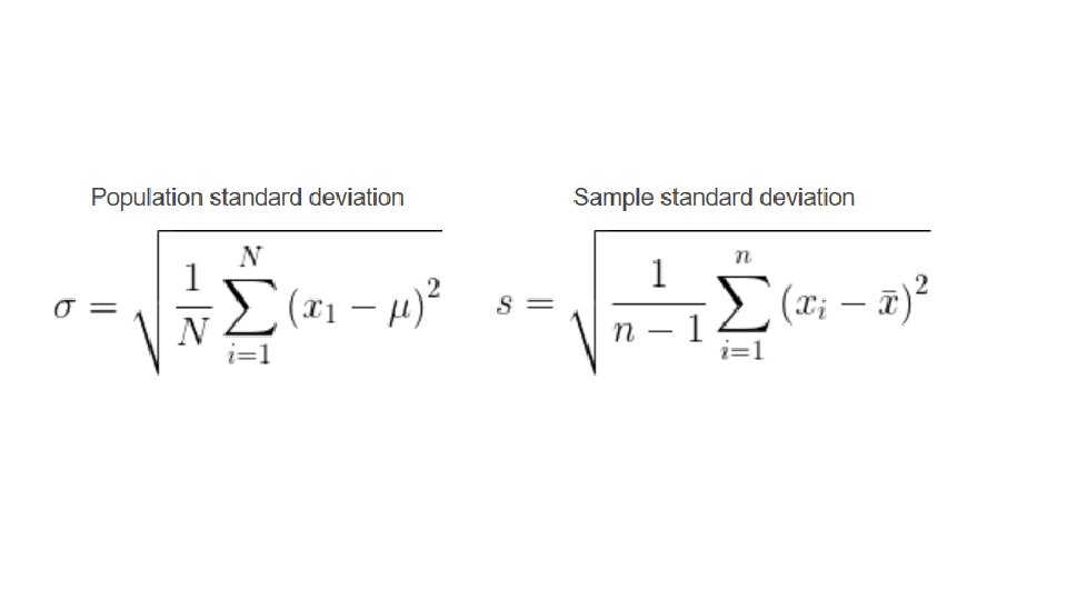
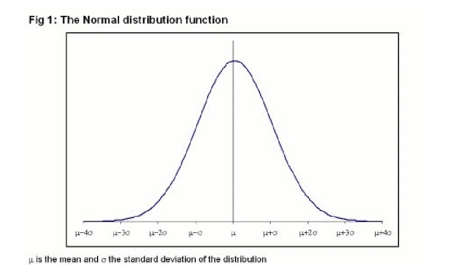
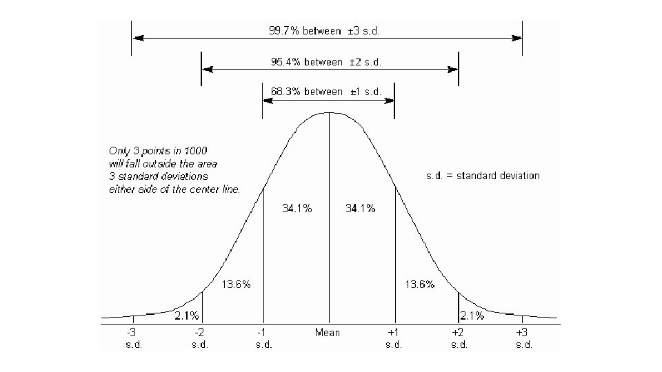
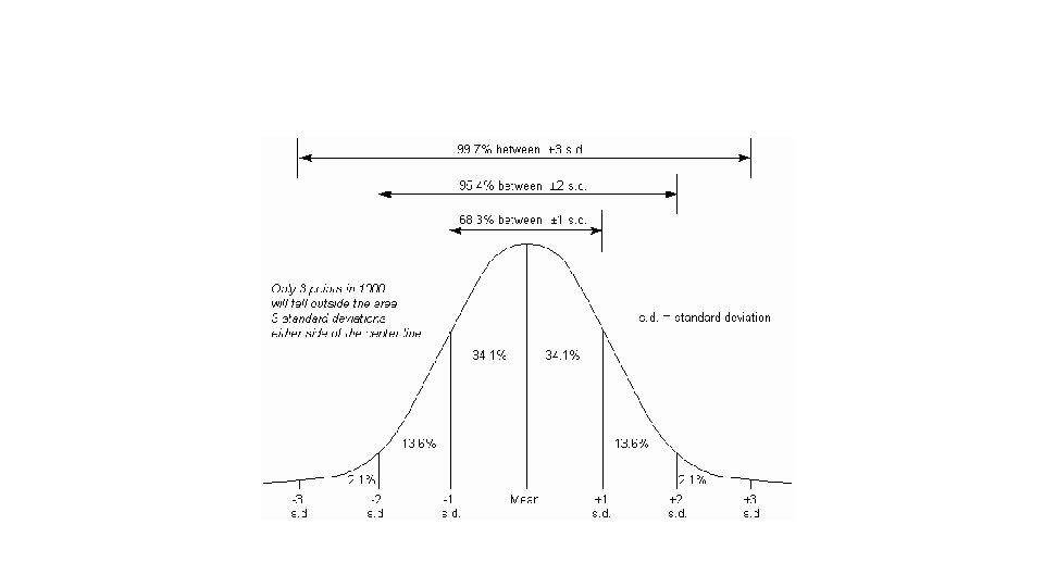
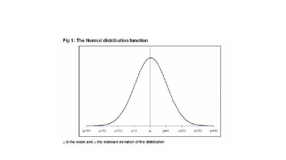
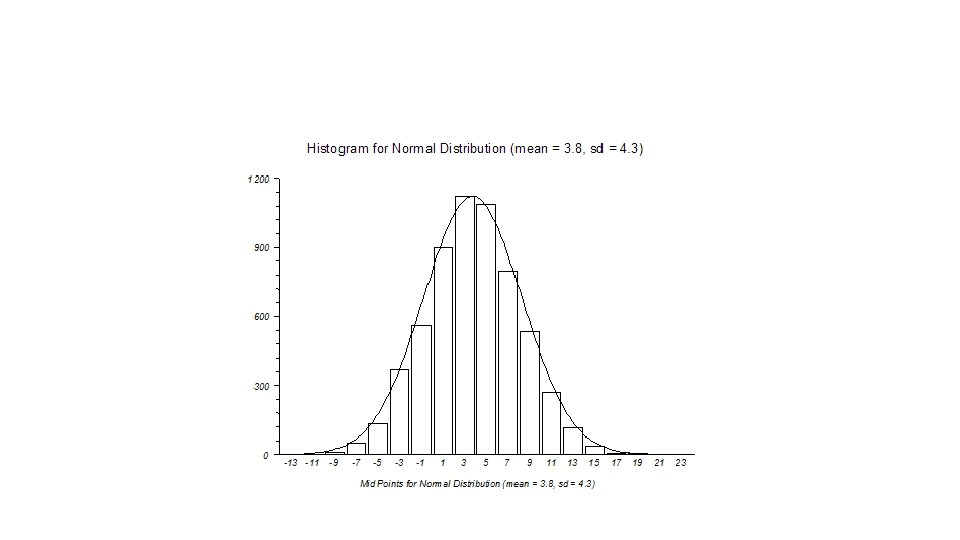
NORMAL DISTRIBUTION MEAN AND STANDARD DEVIATION

DISTRIBUTIONS • For each distribution, look at an image online (wikipedia generally has images) and describe what you see relative to the normal distribution • • Binomial distribution Student’s T distribution Chi-squared distribution Poisson distribution

Confidence Intervals

Uses of Confidence Intervals • Extrapolate a mean from a sample to a population • Identify the set of “most common” or most probable values • Answer benchmarking questions

Confidence Interval Questions • Based on my sample, what range of values would I expect the population mean to fall within? • Based on my sample, what is the set of most probable values for this variable? • Accounting for sampling error, does what we observe match a specific set value (e. g. , a national or competitor average or a benchmark)?

Sample vs. Population • A sample—particularly a randomly selected sample—generally statistically resembles the sampling frame (population) from which it was drawn. • This means that the mean and standard deviation of a sample is generally similar to the mean and standard deviation of the population. • Though good estimates, samples are never identical to the population. • The difference between the sample and the population is called “sampling error. ”

Confidence Interval • A confidence interval is the range of values that is bound by the two values that identify the boundaries between being “likely” to be observed in the population based on a sample and “unlikely” to be observed. • “Likely” and “unlikely” are subjective, and correspond to a particular tolerance for uncertainty. This level of tolerance is called the “confidence level. ” The amount of uncertainty tolerated is called α. • Confidence level + α = 100 • This confidence interval (range of population estimates) is centered on the sample mean or sample proportion.

Confidence and Uncertainty Levels • α represents the uncertainty you are willing to live with. An α of 0. 05 represents a tolerance of 5 percent uncertainty, and corresponds to a 95 % confidence level. This is the standard. • α=0. 10 corresponds to confidence level 90% • α=0. 05 corresponds to confidence level 95% • α=0. 01 corresponds to confidence level 99%

The Distributions in the Background • Because mean values are distributed differently than raw values, they have their own distribution curve. This curve is called the “student’s tdistribution. ” • Unlike a normal curve, the t-distribution shape changes depending on the size of the sample. • The t-distribution can be used to make estimates about the population based on a sample (assuming the sample was drawn randomly) • Similarly, for binary data, we use a binomial distribution to develop confidence intervals.

Introduction to Hypothesis Testing

• Are we likely to observe a particular value in the population based on what we have observed in our sample? • We use probabilities to answer this question, but the answer itself is either a “yes” or “no. ” • One way to answer this question is to see whether the value of interest is inside or outside the confidence interval. • Another way to answer this question uses probabilities.

Using Probabilities to Test a Value (t-test) • What is the probability of observing our (actual, observed) sample if the hypothesized mean (benchmark or comparison value) were the true mean? • This probability is known as the p-value. • If this probability is sufficiently small, (i. e. it is unlikely that we would have observed this value by chance), we say that the value is significantly different from the mean or proportion in our sample and thus unlikely to be the true mean value. • The value for “sufficiently small” is α.

Generating the Results

Descriptive Statistics in Excel • To generate a mean value: =average() • To generate a median value: =median() • To generate the modal value: =mode() • To generate a standard deviation: =stdev. s() • To generate a maximum value: =max() • To generate a minimum value: =min() • To generate a confidence interval for a mean value: =confidence. t()

Z-Scores

• We know everything about the distribution of a normally distributed variable if we know the mean and the standard deviation. • Using these two values, we can figure out how likely we are to observe any value. • This is very useful when we need to standardize decisionmaking

• Let’s call a one standard deviation distance from the mean “z”. • When we count distances from the mean in “z, ” this is called a z-score or a standard normal score.

• You can figure out how many “z”s away from the mean any number is.

• A negative z-score indicates a value below the mean. • A positive z-score indicates a value above the mean. • The normal curve is symmetric, so a z-score of –z has the same probability of occurring as a score of z.

Application of z-scores to your data • Option 1: Create an index variable (weighted or unweighted) • Option 2: Identify a cutoff point based on a probability • Option 3: Identify a probability associated with a cutoff point (or points)

Excel Functions • =standardize (x, mean, standard deviation) returns the z-score for a value in your distribution • =normdist (x, mean, standard deviation, TRUE) returns the probability of returning any number up to and including x • =norminv(probability, mean, standard deviation) returns the value associated with a particular cumulative probability • =normsdist(z) returns the cumulative probability associated with a particular z-score • =normsinv(probability) returns a z-score associated with a particular cumulative probability

Creating an index: Combined scores using zscores • Step 1: Calculate the mean and standard deviation for each variable you want to include in your composite score. • Step 2. Convert each of the raw scores into z-scores using the standardization formula (z=(score-mean)/standard deviation) or Excel (=standardize(score, mean, standard deviation)) • Step 3: Weight the individual subscores, if desired. • Step 4: Add the z-scores for the (weighted) variables you want to include in the composite index score.

Example problem: Garbage collection Crew Tons collected Complaints against A 127 6 B 132 8 C 118 4 D 170 9 E 123 3 Step 1: Calculate mean and standard deviation

Example problem: Garbage collection Crew Tons collected Complaints against A 127 6 B 132 8 C 118 4 D 170 9 E 123 3 Mean 134 6 Standard deviation 18. 6 2. 3 Step 2: Calculate z-scores

Example problem: Garbage collection Crew Tons collected zscore (T) Complaints against Complaints z-score (C) A 127 -. 38 6 0 B 132 -. 11 8 . 87 C 118 -. 86 4 -. 87 D 170 1. 94 9 1. 30 E 123 -. 59 3 -1. 30 Mean 134 6 Standard deviation 18. 6 2. 3 Step 3: Add weights, if desired

Example problem: Garbage collection Crew Tons collected zscore (T) Complaints against Complaints (reversed) z-score (C) A 127 -. 38 6 0 B 132 -. 11 8 -. 87 C 118 -. 86 4 . 87 D 170 1. 94 9 -1. 30 E 123 -. 59 3 1. 30 Mean 134 6 Standard deviation 18. 6 2. 3 Step 4: Add the z-scores to create a composite index

Example problem: Garbage collection Crew Tons collected zscore (T) Complaints against Complaints Equally (reversed) weighted z-score (C) performance score (T+C) A 127 -. 38 6 0 -. 38 B 132 -. 11 8 -. 87 -. 98 C 118 -. 86 4 . 87 . 01 D 170 1. 94 9 -1. 30 . 64 E 123 -. 59 3 1. 30 . 71 Mean 134 6 Standard deviation 18. 6 2. 3 Ta-da! Use these scores to evaluate

Standardizing in R • scale(X, center = TRUE, scale=TRUE)

Standardizing in Excel • Standardize(x)