Lessons Learned from coupling a highresolution weather model

Lessons Learned from coupling a high-resolution weather model with a hydrologic model for flood forecasting Hilary Mc. Millan Associate Professor, Dept of Geography, San Diego State

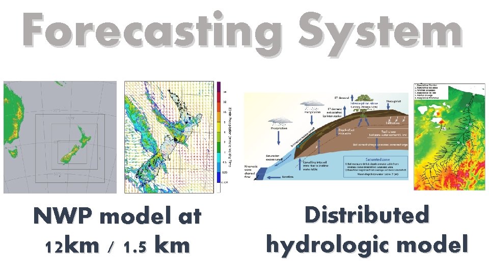
Forecasting System NWP model at 12 km / 1. 5 km Distributed hydrologic model

SCALE BIAS LAG

SCALE

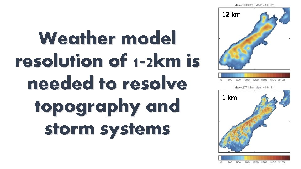
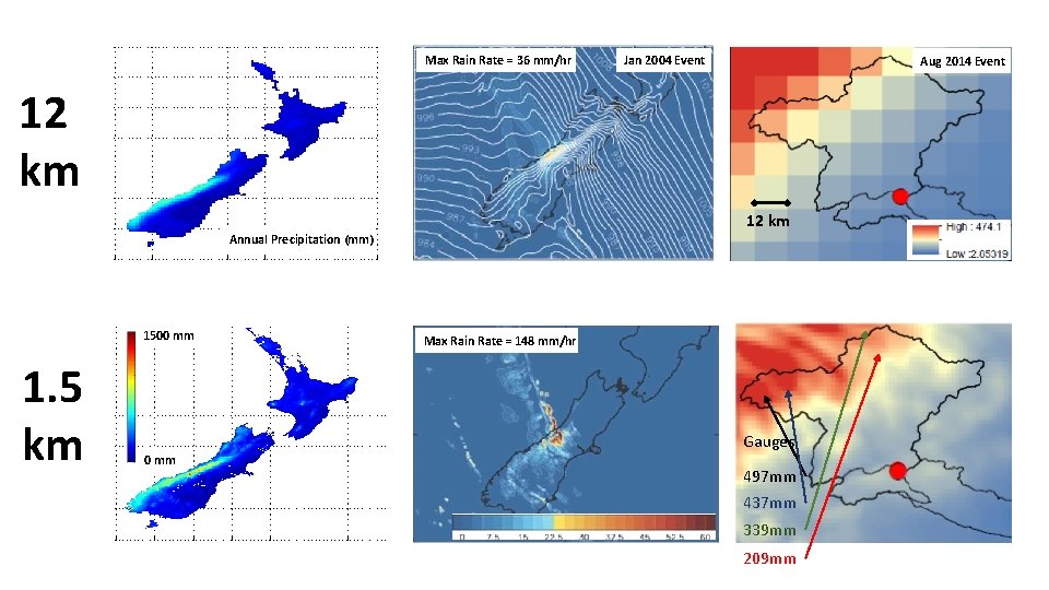
12 km Weather model resolution of 1 -2 km is needed to resolve topography and storm systems 1 km

Max Rain Rate = 36 mm/hr Jan 2004 Event Aug 2014 Event 12 km Annual Precipitation (mm) 1500 mm 1. 5 km Max Rain Rate = 148 mm/hr Gauges 0 mm 497 mm 437 mm 339 mm 209 mm

BIAS

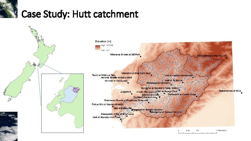
Case Study: Hutt catchment

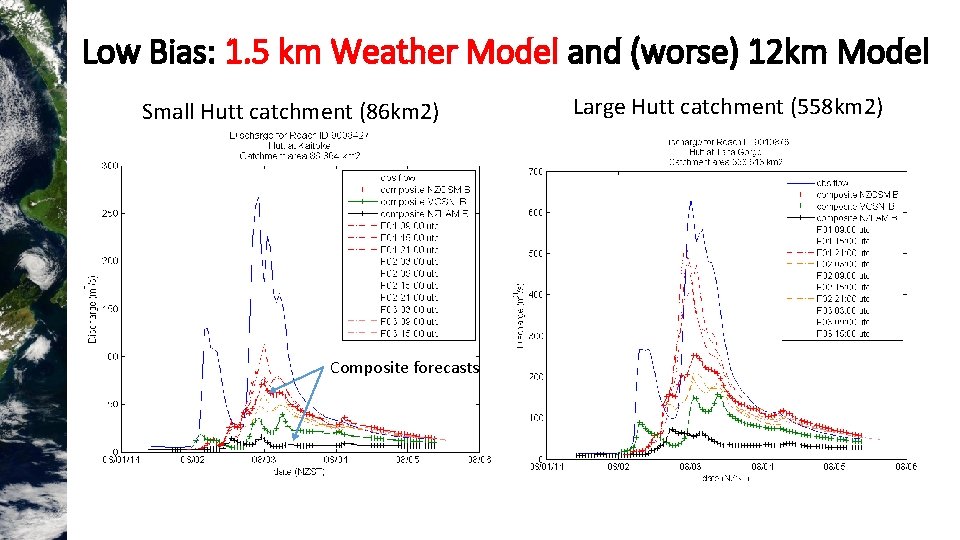
Low Bias: 1. 5 km Weather Model and (worse) 12 km Model Small Hutt catchment (86 km 2) Composite forecasts Large Hutt catchment (558 km 2)

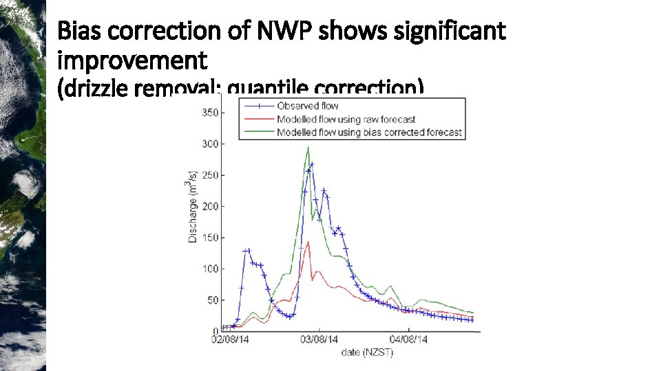
Bias correction of NWP shows significant improvement (drizzle removal; quantile correction)

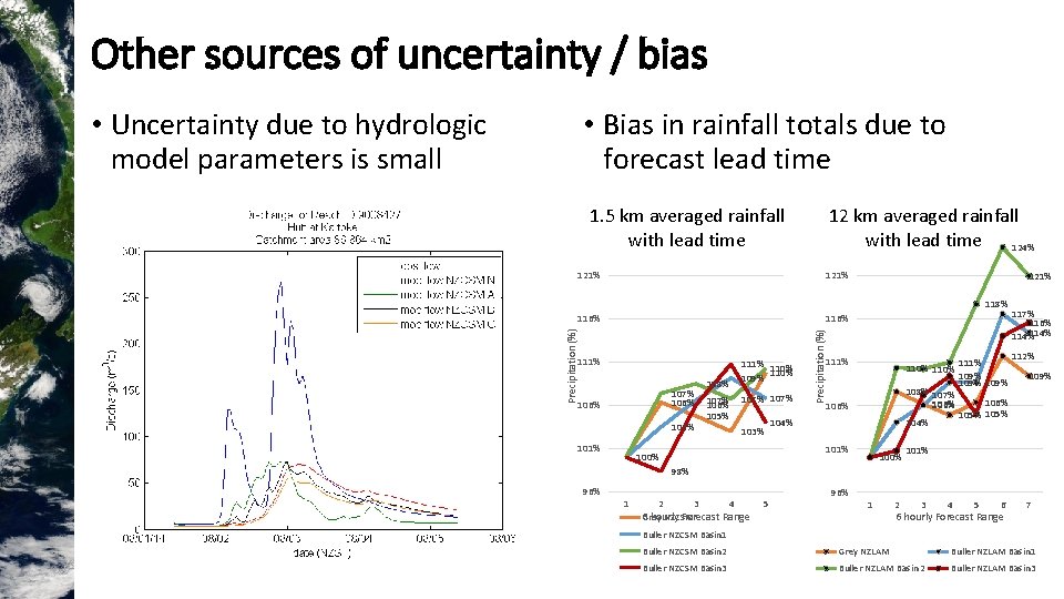
Other sources of uncertainty / bias • Uncertainty due to hydrologic model parameters is small • Bias in rainfall totals due to forecast lead time 12 km averaged rainfall with lead time 124% 1. 5 km averaged rainfall with lead time 121% 116% 121% 111% 107% 106% 103% 101% 108% 107% 106% 105% 111% 110% 109% 107% 103% Precipitation (%) 118% 111% 110% 108% 107% 106% 104% 101% 100% 111% 109% 117% 116% 114% 112% 109% 106% 105% 101% 98% 96% 1 2 3 4 6 Grey hourly Forecast Range NZCSM 5 96% 1 2 3 4 5 6 6 hourly Forecast Range 7 Buller NZCSM Basin 1 Buller NZCSM Basin 2 Grey NZLAM Buller NZLAM Basin 1 Buller NZCSM Basin 3 Buller NZLAM Basin 2 Buller NZLAM Basin 3

LAG

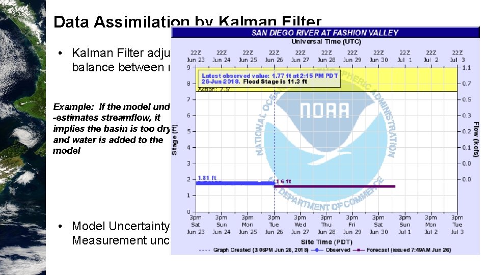
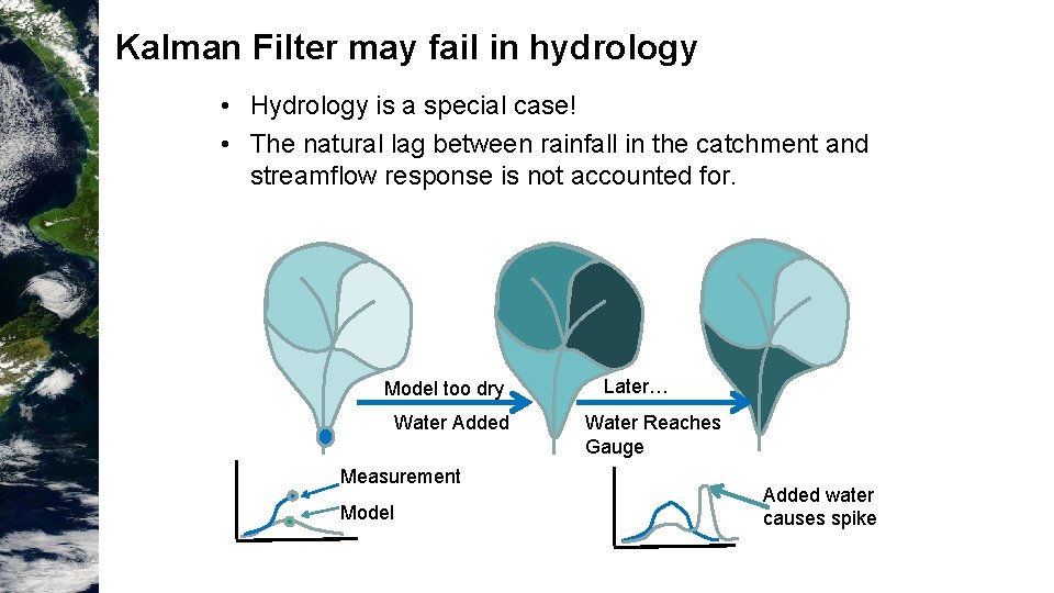
Data Assimilation by Kalman Filter Example: If the model under -estimates streamflow, it implies the basin is too dry, and water is added to the model Flow • Kalman Filter adjusts water volume in model stores, striking the optimal balance between model uncertainty and measurement uncertainty • Model Uncertainty is estimated using an ensemble of model realisations. Measurement uncertainty estimated as fixed percentage of flow.

Kalman Filter may fail in hydrology • Hydrology is a special case! • The natural lag between rainfall in the catchment and streamflow response is not accounted for. Model too dry Water Added Measurement Model Later… Water Reaches Gauge Added water causes spike

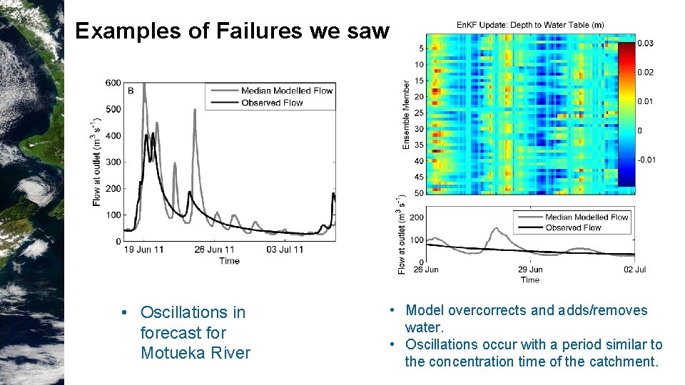
Examples of Failures we saw… • Oscillations in forecast for Motueka River • Model overcorrects and adds/removes water. • Oscillations occur with a period similar to the concentration time of the catchment.

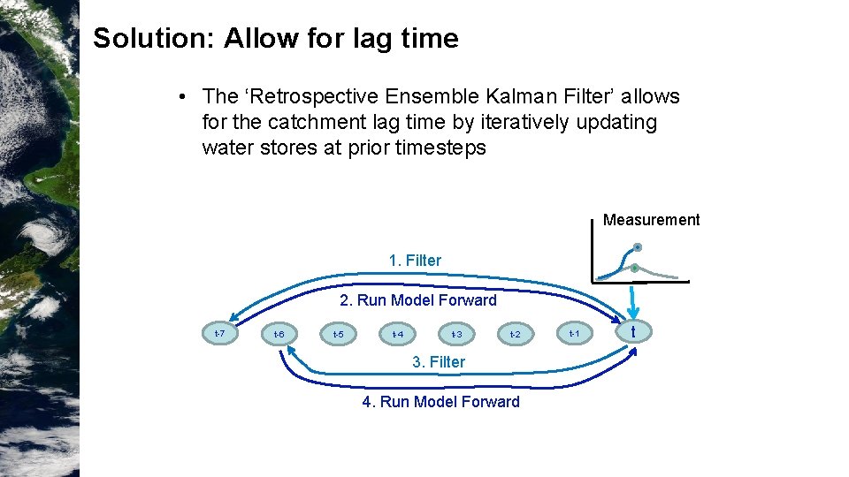
Solution: Allow for lag time • The ‘Retrospective Ensemble Kalman Filter’ allows for the catchment lag time by iteratively updating water stores at prior timesteps Measurement 1. Filter 2. Run Model Forward t-7 t-6 t-5 t-4 t-3 t-2 3. Filter 4. Run Model Forward t-1 t

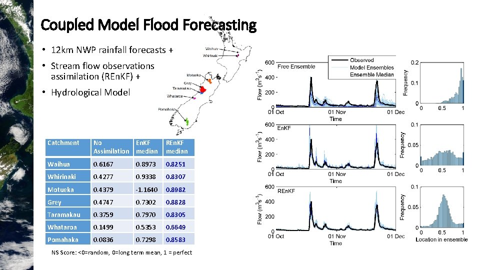
Coupled Model Flood Forecasting • 12 km NWP rainfall forecasts + • Stream flow observations assimilation (REn. KF) + • Hydrological Model Catchment No En. KF Assimilation median REn. KF median Waihua 0. 6167 0. 8973 0. 8251 Whirinaki 0. 4277 0. 9338 0. 8307 Motueka 0. 4379 -1. 1640 0. 8982 Grey 0. 4747 0. 7302 0. 8828 Taramakau 0. 3759 0. 7970 0. 8305 Whataroa 0. 1499 0. 5353 0. 6649 Pomahaka 0. 0836 0. 7298 0. 8583 NS Score: <0=random, 0=long term mean, 1 = perfect

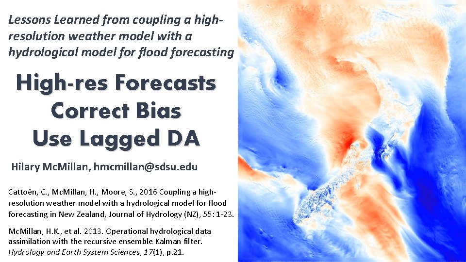
Lessons Learned from coupling a highresolution weather model with a hydrological model for flood forecasting High-res Forecasts Correct Bias Use Lagged DA Hilary Mc. Millan, hmcmillan@sdsu. edu Cattoën, C. , Mc. Millan, H. , Moore, S. , 2016 Coupling a highresolution weather model with a hydrological model for flood forecasting in New Zealand, Journal of Hydrology (NZ), 55: 1 -23. Mc. Millan, H. K. , et al. 2013. Operational hydrological data assimilation with the recursive ensemble Kalman filter. Hydrology and Earth System Sciences, 17(1), p. 21.