Lessons Introduction to Data Structures Computer Memory Pointers

Lessons: • • Introduction to Data Structures Computer Memory Pointers and Indirection Linear Data Structures – – – • Nonlinear Data Structures – – – • • Ordered List: The Abstract View Ordered List: The Implementation View Stacks: The Abstract View Stacks: The Implementation View Queues: The Abstract View Queues: The Implementation View Multidimensional arrays Trees Graphs Abstract Data Types Summary created on 29/10/2008 yahaya. wordpress. com 1

Learning objectives: • Show data structures map onto physical memory. • Identify linear versus nonlinear data structures. • Manipulate data structures with basic operations. • Compare different implementations of the same data structure. created on 29/10/2008 yahaya. wordpress. com 2

Introduction: • The following lessons introduce the topic of data structures by comparing how data is actually stored in a computer with the abstract structures that programmers use. To illustrate this comparison, several basic data structures such as lists, stacks, and queues are described. Each lesson includes a set of review questions which test the important concepts from the lesson and provide practice problems. After reading each lesson, you should work the review questions before proceeding to the next lesson. Use the navigation bar at the top of this page to view the lessons and access the review questions. Each lesson page has a link on the navigation bar which will take you to the review questions for that lesson. To begin your study, click at the top of this page. • created on 29/10/2008 yahaya. wordpress. com 3

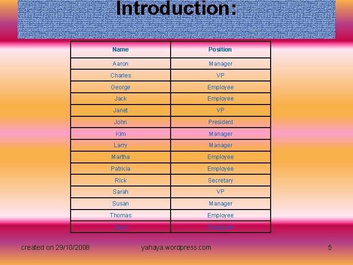
Introduction: • Imagine that you are hired by company XYZ to organize all of their records into a computer database. The first thing you are asked to do is create a database of names with all the company's management and employees. To start your work, you make a list of everyone in the company along with their position. created on 29/10/2008 yahaya. wordpress. com 4

Introduction: created on 29/10/2008 Name Position Aaron Manager Charles VP George Employee Jack Employee Janet VP John President Kim Manager Larry Manager Martha Employee Patricia Employee Rick Secretary Sarah VP Susan Manager Thomas Employee Zack Employee yahaya. wordpress. com 5

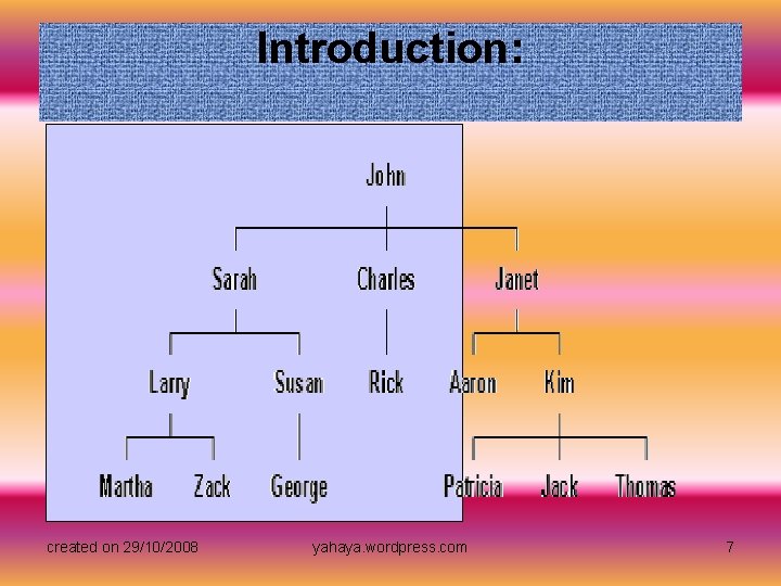
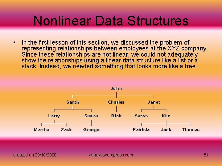
Introduction: • But this list only shows one view of the company. You also want your database to represent the relationships between management and employees at XYZ. Although your list contains both name and position, it does not tell you which managers are responsible for which workers and so on. After thinking about the problem for a while, you decide that a tree diagram is a much better structure for showing the work relationships at XYZ. created on 29/10/2008 yahaya. wordpress. com 6

Introduction: created on 29/10/2008 yahaya. wordpress. com 7

Introduction: • These two diagrams are examples of different data structures. In one of the data structures, your data is organized into a list. This is very useful for keeping the names of the employees in alphabetical order so that we can locate the employee's record very quickly. However, this structure is not very useful for showing the relationships between employees. A tree structure is much better suited for this purpose. • In computer science, data structures are an important way of organizing information in a computer. Just like the diagrams above illustrate, there are many different data structures that programmers use to organize data in computers. Some data structures are similar to the tree diagram because they are good for representing relationships between data. Other structures are good for ordering data in a particular way like the list of employees. Each data structure has unique properties that make it well suited to give a certain view of the data. created on 29/10/2008 yahaya. wordpress. com 8

Introduction: • During these lessons, you will learn how data structures are created inside a computer. You will find there is quite a difference between your mental picture of a data structure and the actual way a computer stores a data structure in memory. You will also discover that there are many different ways of creating the same data structure in a computer. These various approaches are tradeoffs that programmers must consider when writing software. Finally, you will see that each data structure has certain operations that naturally fit with the data structure. Often these operations are bundled with the data structure and together they are called a data type. By the end of this study, you should be able to do the following: created on 29/10/2008 yahaya. wordpress. com 9

Introduction: • Show data structures are represented in the computer, • Identify linear and nonlinear data structures, • Manipulate data structures with basic operations, and • Compare different implementations of the same data structure created on 29/10/2008 yahaya. wordpress. com 10

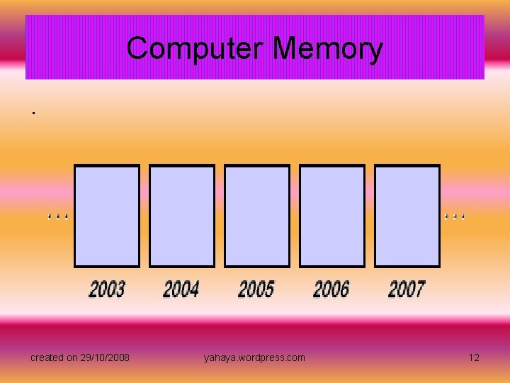
Computer Memory • To understand how a computer can represents large data structures like our tree diagram, we first need to understand some basic facts about computer memory. Every piece of data that is stored in a computer is kept in a memory cell with a specific address. We can think of these memory cells as being a long row of boxes where each box is labeled with an address. If you have ever used a computer spreadsheet before, you know that spreadsheets also have labeled boxes that can hold data. Computer memory is similar to this with the exception that computer memory is linear. That's why we think of computer memory as being organized in a row rather than a grid like a spreadsheet. created on 29/10/2008 yahaya. wordpress. com 11

Computer Memory. created on 29/10/2008 yahaya. wordpress. com 12

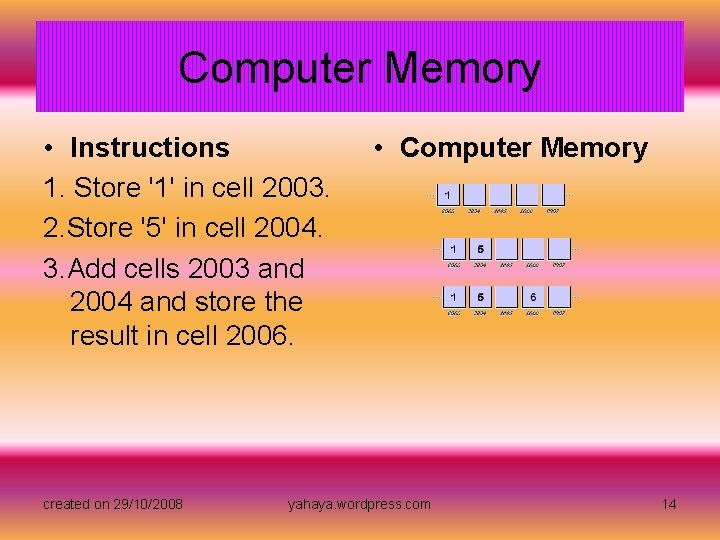
Computer Memory • The computer can store many different types of data in its memory. You have already learned about some of the basic types of data the computer uses. These include integers, real numbers, and characters. Once the computer stores data in the memory cells, it can access the data by using the address of the data cells. For example, consider the following instructions for adding two integers together. created on 29/10/2008 yahaya. wordpress. com 13

Computer Memory • Instructions 1. Store '1' in cell 2003. 2. Store '5' in cell 2004. 3. Add cells 2003 and 2004 and store the result in cell 2006. created on 29/10/2008 • Computer Memory yahaya. wordpress. com 14

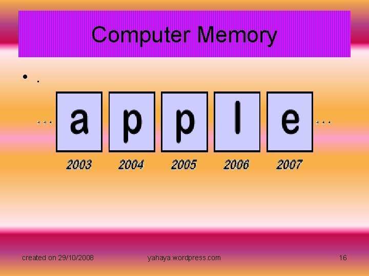
Computer Memory • Notice how the computer performs operations by referring to the address of the memory cells. These addresses are a very important component in creating various data structures in computer memory. For example, suppose we want a data structure that can store a group of characters as a word. In many computer languages, this data structure is called a string. If we store the characters for the string 'apple' in the computer's memory, it might look something like this. created on 29/10/2008 yahaya. wordpress. com 15

Computer Memory • . created on 29/10/2008 yahaya. wordpress. com 16

Computer Memory • In order for the computer to recognize that 'apple' is a string, it must have some way of identifying the start and end of the characters stored in memory. This is why the addresses of the memory cells are important. By using the addresses to refer to a group of memory cells as a string, the computer can store many strings in a row to create a list. This is one way that we could create a data structure to represent our list of employees at company XYZ. created on 29/10/2008 yahaya. wordpress. com 17

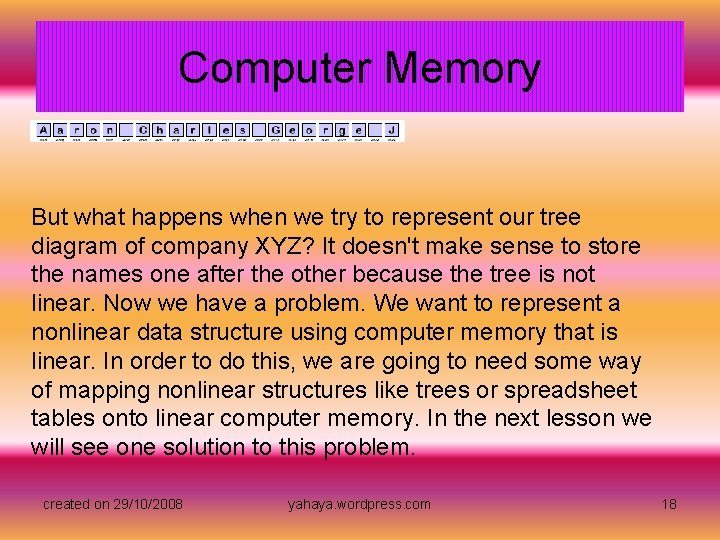
Computer Memory But what happens when we try to represent our tree diagram of company XYZ? It doesn't make sense to store the names one after the other because the tree is not linear. Now we have a problem. We want to represent a nonlinear data structure using computer memory that is linear. In order to do this, we are going to need some way of mapping nonlinear structures like trees or spreadsheet tables onto linear computer memory. In the next lesson we will see one solution to this problem. created on 29/10/2008 yahaya. wordpress. com 18

Pointers and Indirection • In our last lesson, we discovered a problem with representing data structures that are not linear. We need some way to map these data structures to the computer's linear memory. One solution is to use pointers. Pointers are memory locations that are stored in memory cells. By using a pointer, one memory cell can "point" to another memory cell by holding a memory address rather than data. Let's see how it works. created on 29/10/2008 yahaya. wordpress. com 19

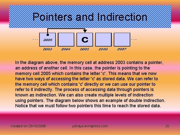
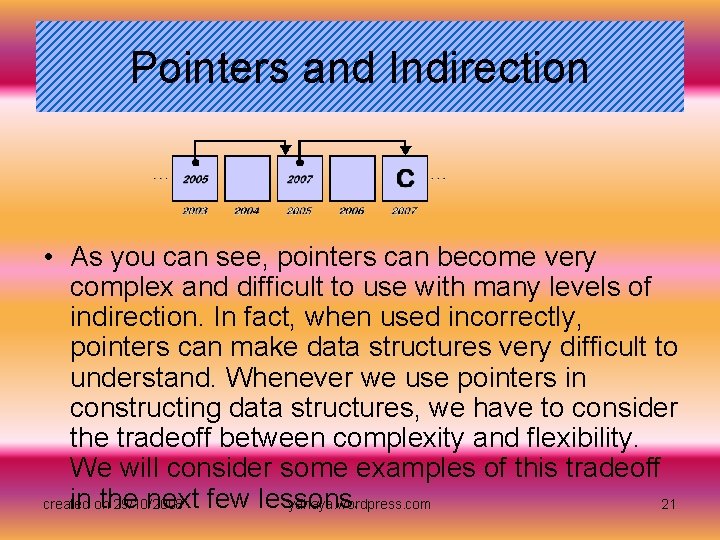
Pointers and Indirection In the diagram above, the memory cell at address 2003 contains a pointer, an address of another cell. In this case, the pointer is pointing to the memory cell 2005 which contains the letter 'c'. This means that we now have two ways of accessing the letter 'c' as stored data. We can refer to the memory cell which contains 'c' directly or we can use our pointer to refer to it indirectly. The process of accessing data through pointers is known as indirection. We can also create multiple levels of indirection using pointers. The diagram below shows an example of double indirection. Notice that we must follow two pointers this time to reach the stored data. created on 29/10/2008 yahaya. wordpress. com 20

Pointers and Indirection • As you can see, pointers can become very complex and difficult to use with many levels of indirection. In fact, when used incorrectly, pointers can make data structures very difficult to understand. Whenever we use pointers in constructing data structures, we have to consider the tradeoff between complexity and flexibility. We will consider some examples of this tradeoff in onthe next few lessons. created 29/10/2008 yahaya. wordpress. com 21

Pointers and Indirection • The idea of pointers and indirection is not exclusive to computer memory. Pointers appear in many different aspects of computer use. A good example is hyperlinks in web pages. This links are really pointers to another web page. Perhaps you have even experienced "double indirection" when you went to visit a familiar web site and found the site had moved. Instead of the page you expected, you saw a notice that the web pages had been moved and a link to the new site. Rather than clicking a single link, you had to follow two links or two pointers to reach the web page. created on 29/10/2008 yahaya. wordpress. com 22

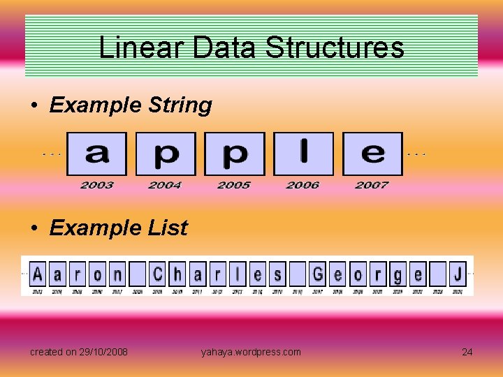
Linear Data Structures • In our previous lesson, we saw that it is very simple to create data structures that are organized similar to the way the computer's memory is organized. For example, the list of employee's from the XYZ company is a linear data structure. Since the computer's memory is also linear, it is very easy to see how we can represent this list with the computer. Any data structure which organizes the data elements one after the other is a linear data structure. So far we have seen two examples of linear data structures: the string data structure (a list of characters) and the XYZ company list (a list of strings). created on 29/10/2008 yahaya. wordpress. com 23

Linear Data Structures • Example String • Example List created on 29/10/2008 yahaya. wordpress. com 24

Linear Data Structures • You may have noticed that these two examples of linear data structures resemble each other. This is because they are both really different kinds of lists. In general, all linear data structures look like a list. However, this does not mean that all linear data structures are exactly the same. Suppose I want to design a list to store the names of the XYZ employees in the computer. One possible design is to organize the names similar to the example picture above. Another possible design is to use the pointers we learned about in the last lesson. While these two designs provide the same functionality (i. e. a list that can hold names), the way they are implemented in the computer is much different. This means that there is an abstract view of a list which is distinct from any particular computer implementation. We will return to this idea of an abstract view of a data structure in the next few lessons. created on 29/10/2008 yahaya. wordpress. com 25

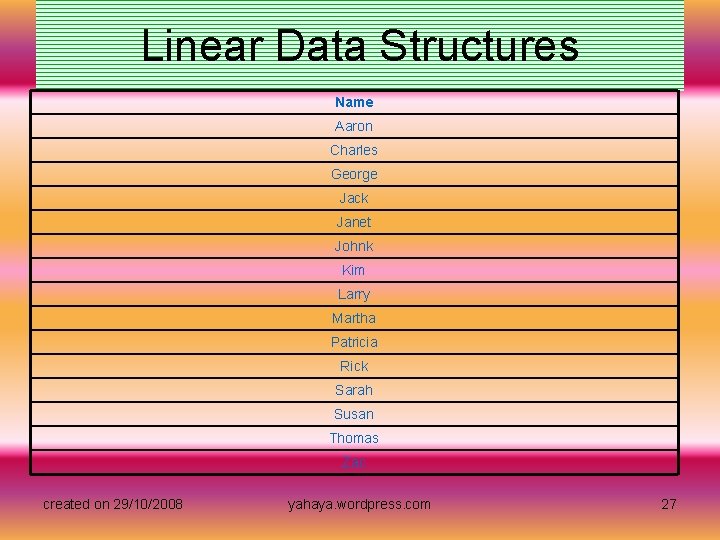
Linear Data Structures • You may have also noticed that the example picture of the XYZ employees is not exactly the same as the original list. Take another look at the employee list to the right. When we make a list of names, we tend to organize this list in a column rather than a row. In this case, the conceptual or logical representation of a list is a column of names. However, the physical representation of the list in the computer's memory is a row of strings. For most data structures, the way that we think about them is far different from the way they are implemented in the computer. In other words, the physical representation is much different than the logical representation, especially in data structures that use pointers. created on 29/10/2008 yahaya. wordpress. com 26

Linear Data Structures Name Aaron Charles George Jack Janet Johnk Kim Larry Martha Patricia Rick Sarah Susan Thomas Zac created on 29/10/2008 yahaya. wordpress. com 27

Linear Data Structures • During the next few lessons, we will examine several different linear data structures with a focus on the following ideas: • The abstract view versus the implementation • The logical representation verses the physical representation • Comparison of various implementations created on 29/10/2008 yahaya. wordpress. com 28

Ordered List: The Abstract View • • The most common linear data structure is the list. By now you are already pretty familiar with the idea of a list and at least one way of representing a list in the computer. Now we are going to look at a particular kind of list: an ordered list. Ordered lists are very similar to the alphabetical list of employee names for the XYZ company. These lists keep items in a specific order such as alphabetical or numerical order. Whenever an item is added to the list, it is placed in the correct sorted position so that the entire list is always sorted. Before we consider how to implement such a list, we need to consider the abstract view of an ordered list. Since the idea of an abstract view of a list may be a little confusing, let's think about a more familiar example. Consider the abstract view of a television. Regardless of who makes a television, we all expect certain basic things like the ability to change channels and adjust the volume. As long as these operations are available and the TV displays the shows we want to view, we really don't care about who made the TV or how they chose to construct it. The circuitry inside the TV set may be very different from one brand to the next, but the functionality remains the same. Similarly, when we consider the abstract view of an ordered list, we don't worry about the details of implementation. We are only concerned with what the list does, not how it does it. created on 29/10/2008 yahaya. wordpress. com 29

Ordered List: The Abstract View • Suppose we want a list that can hold the following group of sorted numbers: [2 4 6 7]. What are some things that we might want to do with our list? Well, since our list is in order, we will need some way of adding numbers to the list in the proper place, and we will need some way of deleting numbers we don't want from the list. To represent these operations, we will use the following notation: • Add. List. Item(List, Item) Remove. List. Item(List, Item) • Each operation has a name and a list of parameters the operation needs. The parameter list for the Add. List. Item operation includes a list (the list we want to add to) and an item (the item we want to add). The Remove. List. Item operation is very similar except this time we specify the item we want to remove. These operations are part of the abstract view of an ordered list. They are what we expect from any ordered list regardless of how it is implemented in the computer. created on 29/10/2008 yahaya. wordpress. com 30

Ordered List: The Implementation • In this lesson, we are going to look at two different ways of creating an ordered list data structure to hold the following list [2 4 6 7]. First, we will create a list using an array of memory cells. Next, we will create the same list using pointers. Finally, we will compare these two approaches to see the advantages and disadvantages. • Array Implementation • One approach to creating a list is simply to reserve a block of adjacent memory cells large enough to hold the entire list. Such a block of memory is called an array. Of course, since we will want to add items to our list, we need to reserve more than just four memory cells. For now, we will make our array large enough to hold six numbers. The animation below shows a graphical representation of our array in memory with the list numbers. Follow the directions in the animation to learn how the list operations Add. List. Item and Remove. List. Item work. created on 29/10/2008 yahaya. wordpress. com 31

Ordered List: The Implementation • In the animation, you saw that there were two disadvantages to using an array to implement an ordered list. First, you saw that the elements in the list must be kept in sequence, that is, there must not be gaps in the list. If gaps are allowed, the computer will not be able to determine which items are part of the list and which items are not. For this reason, the ordered list structures that are implemented with arrays are known as sequential lists. • The second disadvantage that you saw was that arrays have a fixed size and therefore limit the number of items the list can contain. Of course we could try to increase the size of the array, but it may not always be the case that the adjacent memory cells in the computer are available. They could be in use by some other program. However, it is quite likely that the computer does have available memory at some other non-adjacent location. To take advantage of this memory, we need to design our list so that the list items do not have to be adjacent. created on 29/10/2008 yahaya. wordpress. com 32

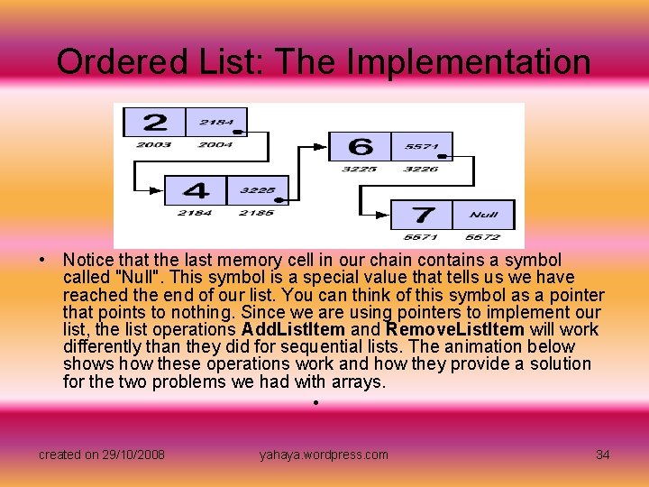
Ordered List: The Implementation • Pointer Implementation • A second approach to creating a list is to link groups of memory cells together using pointers. Each group of memory cells is called a node. With this implementation every node contains a data item and a pointer to the next item in the list. You can picture this structure as a chain of nodes linked together by pointers. As long as we know where the chain begins, we can follow the links to reach any item in the list. Often this structure is called a linked list. created on 29/10/2008 yahaya. wordpress. com 33

Ordered List: The Implementation • Notice that the last memory cell in our chain contains a symbol called "Null". This symbol is a special value that tells us we have reached the end of our list. You can think of this symbol as a pointer that points to nothing. Since we are using pointers to implement our list, the list operations Add. List. Item and Remove. List. Item will work differently than they did for sequential lists. The animation below shows how these operations work and how they provide a solution for the two problems we had with arrays. • created on 29/10/2008 yahaya. wordpress. com 34

Ordered List: The Implementation • By implementing our list with pointers, we are able to avoid the two disadvantages we discovered with using sequential lists. However, this does not mean that linked lists are the perfect solution. Whenever we use indirection in building a data structure, it becomes much harder to find mistakes. For example, it is very easy to assign the wrong address to a pointer and "short circuit" our list. In general, sequential lists are simpler than linked lists but they are also more limited. Linked lists give us a great amount of flexibility but this comes at the cost of increased complexity created on 29/10/2008 yahaya. wordpress. com 35

Stacks: The Abstract View • Another common linear data structure is the stack. Just like we did with the ordered list, we will examine the abstract view of a stack first and then look at a couple of ways a stack can be implemented. In one way, a stack is very similar to a list except that a stack is more restricted. The animation below should give you a good idea of the abstract view of a stack. Follow the directions to manipulate a simple stack and learn about the operations that a stack provides. created on 29/10/2008 yahaya. wordpress. com 36

Stacks: The Abstract View • Now that you know how a stack works, you can see that this data structure is really a restricted list. With the stack, we have restricted the access to one end of the list by using the pop and push operations. The result of this restriction is that items in the list pile on top of the other. To get to the bottom item, we must first remove all the items above it. This behavior is sometimes described as "last-in, first-out" or LIFO since the last item to enter the stack is the first item to leave the stack. With the stack, the top item is always the last item to enter the stack and it is always the first item to leave the stack since no other items can be removed until the top item is removed. • Let's take another look at the operations that can be performed on a stack. We will represent these two operations with the following notation created on 29/10/2008 yahaya. wordpress. com 37

Stacks: The Abstract View • Item Push. Stack. Item(Stack, Item) Item Pop. Stack. Item(Stack) • The Push. Stack. Item operation has two parameters which are a stack and an item. This operation adds the item to the top of the specified stack. The Pop. Stack. Item operation only takes one parameter which is a stack. However, notice that this operation has the keyword Item listed to the left. This keyword represents the item that is removed from the top of the stack when the Pop. Stack. Item operation is done. These two operations are part of the abstract view of a stack. They are what we expect from any stack regardless of how it is implemented in the computer. created on 29/10/2008 yahaya. wordpress. com 38

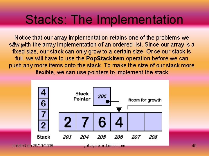
Stacks: The Implementation • As we did with the ordered list, we are going to look at two implementations of a stack. The first implementation uses an array to create the stack data structure, and the second implementation uses pointers. • Array Implementation • In order to implement a stack using an array, we need to reserve a block of memory cells large enough to hold all the items we want to put on the stack. The picture below shows an array of six memory cells that represent our stack. Notice that we have one other memory cell called a stack pointer that holds the location of the top of our stack. As the stack grows and shrinks, this pointer is updated so that it always points to the top item of the stack. created on 29/10/2008 yahaya. wordpress. com 39

Stacks: The Implementation Notice that our array implementation retains one of the problems we saw with the array implementation of an ordered list. Since our array is a fixed size, our stack can only grow to a certain size. Once our stack is full, we will have to use the Pop. Stack. Item operation before we can push any more items onto the stack. To make the size of our stack more flexible, we can use pointers to implement the stack • , created on 29/10/2008 yahaya. wordpress. com 40

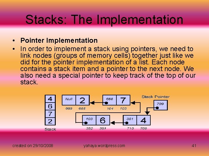
Stacks: The Implementation • Pointer Implementation • In order to implement a stack using pointers, we need to link nodes (groups of memory cells) together just like we did for the pointer implementation of a list. Each node contains a stack item and a pointer to the next node. We also need a special pointer to keep track of the top of our stack. created on 29/10/2008 yahaya. wordpress. com 41

Stacks: The Implementation • Notice that the stack operations can get a little tricky when we use pointers. To push an item onto the stack, we need to find a free memory location, set the pointer of the new location to the top of the stack, and finally set the stack pointer to the new location. The order of these operations is very important. If we set the stack pointer to the location of the new memory first, we will lose the location of the top of our stack. This example shows the same tradeoff that we saw earlier with the ordered list implementations. While the array implementation is simpler, the added complexity of the pointer implementation gives us a more flexible stack. created on 29/10/2008 yahaya. wordpress. com 42

Queues: The Abstract View • The final linear data structure that we will examine is the queue. Like the stack, the queue is a type of restricted list. However, instead of restricting all the operations to one end of the list as a stack does, the queue allows items to be added at one end of the list and removed at the other end. The animation below should give you a good idea of the abstract view of a queue. Follow the directions to manipulate a simple queue and learn about the operations that a queue provides. created on 29/10/2008 yahaya. wordpress. com 43

Queues: The Abstract View • The restrictions placed on a queue cause this structure to be a "first-in, first-out" or FIFO structure. This idea is similar to customer lines at a grocery store. When customer X is ready to check out, he or she enters the tail of the waiting line. When the preceding customers have paid, then customer X pays and exits the head of the line. The check-out line is really a queue that enforces a "first come, first serve" policy. • Now let's take another look at the operations that can be performed on a queue. We will represent these two operations with the following notation created on 29/10/2008 yahaya. wordpress. com 44

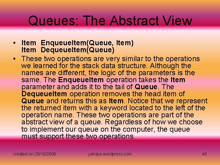
Queues: The Abstract View • Item Enqueue. Item(Queue, Item) Item Dequeue. Item(Queue) • These two operations are very similar to the operations we learned for the stack data structure. Although the names are different, the logic of the parameters is the same. The Enqueue. Item operation takes the Item parameter and adds it to the tail of Queue. The Dequeue. Item operation removes the head item of Queue and returns this as Item. Notice that we represent the returned item with a keyword located to the left of the operation name. These two operations are part of the abstract view of a queue. Regardless of how we choose to implement our queue on the computer, the queue must support these two operations. created on 29/10/2008 yahaya. wordpress. com 45

Queues: The Implementation View • When we looked at the ordered list and stack data structures, we saw two different ways to implement each one. Although the implementations were different, the data structure was still the same from the abstract point of view. We could still use the same operations on the data structures regardless of their implementations. With the queue, it is also possible to have various implementations that support the operations Enqueue. Item and Dequeue. Item. However, in this lesson, we are only going to focus on one implementation in order to highlight another distinction: the distinction between the logical representation of a queue and the physical representation of a queue. Remember that the logical representation is the way that we think of the data being stored in the computer. The physical representation is the way the data is actually organized in the memory cells. created on 29/10/2008 yahaya. wordpress. com 46

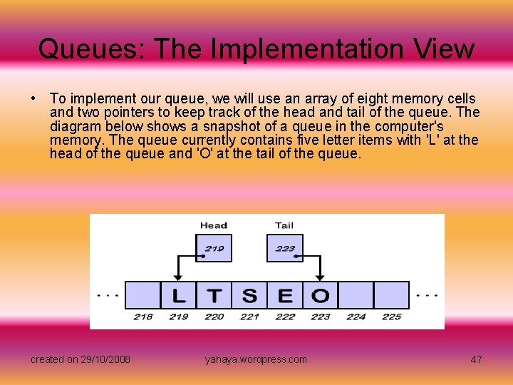
Queues: The Implementation View • To implement our queue, we will use an array of eight memory cells and two pointers to keep track of the head and tail of the queue. The diagram below shows a snapshot of a queue in the computer's memory. The queue currently contains five letter items with 'L' at the head of the queue and 'O' at the tail of the queue. created on 29/10/2008 yahaya. wordpress. com 47

Queues: The Implementation View • Now let's consider how the Enqueue. Item and Dequeue. Item operations might be implemented. To enqueue letters into the queue, we could advance the tail pointer one location and add the new letter. To dequeue letters, we could remove the head letter and increase the head pointer one location. While this approach seems very straightforward, it has a serious problem. As items are added and removed, our queue will march straight through the computer's entire memory. We have not limited the size of our queue. • Perhaps we could limit the size of the queue by not allowing the tail pointer to advance beyond a certain location. This implementation would stop the queue from traversing the entire memory, but it would only allow us to fill the queue one time. Once the head and tail pointers reached the stop location, our queue would no longer work. created on 29/10/2008 yahaya. wordpress. com 48

Queues: The Implementation View • What we really need is a way to make our array circular. Of course, we know that the computer's memory is linear, so we can't change the physical representation of the data. However, we can implement our operations in such a way that our queue acts like it was a ring or a circle. In other words, we are going to create a logical representation that is different from the physical representation in memory. The applet below shows these two representations along with the abstract view of the queue. Click the button below to start the applet. The applet will open in a new window along with instructions for using the queue. created on 29/10/2008 yahaya. wordpress. com 49

Nonlinear Data Structures created on 29/10/2008 yahaya. wordpress. com 50

Nonlinear Data Structures • In the first lesson of this section, we discussed the problem of representing relationships between employees at the XYZ company. Since these relationships are not linear, we could not adequately show the relationships using a linear data structure like a list or a stack. Instead, we needed something that looks more like a tree. created on 29/10/2008 yahaya. wordpress. com 51

Nonlinear Data Structures • A tree is just one example of a nonlinear data structure. Two other examples are multidimensional arrays and graphs. In the next few lessons, we will examine these data structures to see how they are represented using the computer's linear memory. Remember that in the last lesson we saw that we could create a logical representation of a circular queue. Although the actual memory locations were just an array (a group of linear memory cells), we made them seem to be circular by wrapping our pointers around to the front of the array each time they reached the end. This example demonstrated that there are two ways of representing our data structure. The logical representation was a circle or a loop, while the physical representation was a simple linear array. • For each of the data structures we examine, we will look at a simplementation for the data structure to see how it can be represented in physical memory. Then we will compare this physical representation with the logical representation of the data structure created on 29/10/2008 yahaya. wordpress. com 52

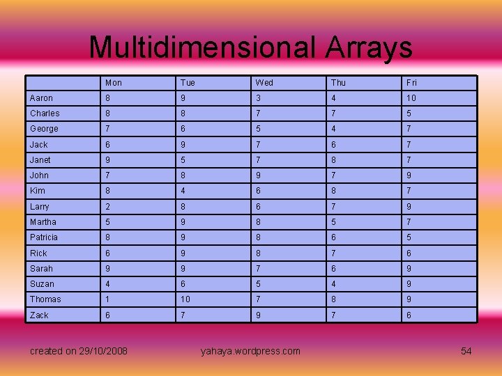
Multidimensional Arrays • Let's return to our example of the XYZ company. After you finish creating a list of the company's employees, you are asked to make an electronic time sheet that shows the number of hours that each employee worked during the week. You begin by associating each data point (hours worked) with two labels: employee's name and day of the week. To organize the data, you use the following logical representation. created on 29/10/2008 yahaya. wordpress. com 53

Multidimensional Arrays Mon Tue Wed Thu Fri Aaron 8 9 3 4 10 Charles 8 8 7 7 5 George 7 6 5 4 7 Jack 6 9 7 6 7 Janet 9 5 7 8 7 John 7 8 9 7 9 Kim 8 4 6 8 7 Larry 2 8 6 7 9 Martha 5 9 8 5 7 Patricia 8 9 8 6 5 Rick 6 9 8 7 6 Sarah 9 9 7 6 9 Suzan 4 6 5 4 9 Thomas 1 10 7 8 9 Zack 6 7 9 7 6 created on 29/10/2008 yahaya. wordpress. com 54

Multidimensional Arrays • Now we have a new data structure called a two-dimensional array. We can see how the data structure gets its name by comparing it with a typical array. All the arrays we have seen so far were simply a group of contiguous memory cells. Since computer memory is linear, the arrays were also linear or one-dimensional. Notice, however, that each row of the table above looks like a typical, linear array. Our table is really a collection of one-dimensional arrays with five memory cells. Each memory cell represents a day of the week, and each array in the table represents an employee. Just like a onedimensional array is a collection of memory cells, a two-dimensional array is a collection of one-dimensional arrays. • You may be wondering how we can represent our two-dimensional array in the computer's memory. The animation below shows the answer to this question by comparing the logical representation (the table) with the physical representation in memory created on 29/10/2008 yahaya. wordpress. com 55

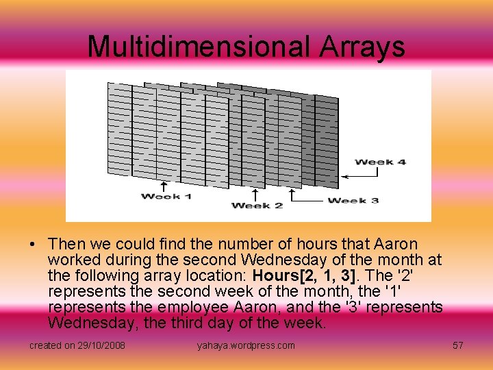
Multidimensional Arrays • As you saw in the animation, it is common to refer to array locations by specifying the row and column numbers after the array name. If we named our table above "Hours" then we could find the number of hours that Aaron worked on Wednesday at the following array location: Hours[1, 3]. • We can also have higher dimensional arrays that are collections of lower dimensional arrays. For example, we could organize the time sheet for one month by making a three-dimensional array. This array would be a collection of four weeks of time sheets which are two-dimensional arrays. created on 29/10/2008 yahaya. wordpress. com 56

Multidimensional Arrays • Then we could find the number of hours that Aaron worked during the second Wednesday of the month at the following array location: Hours[2, 1, 3]. The '2' represents the second week of the month, the '1' represents the employee Aaron, and the '3' represents Wednesday, the third day of the week. created on 29/10/2008 yahaya. wordpress. com 57

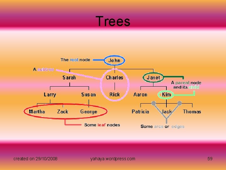
Trees • Another common nonlinear data structure is the tree. We have already seen an example of a tree when we looked at the employee hierarchy from the XYZ company. Let's take another look at this diagram with some of the important features of trees highlighted. created on 29/10/2008 yahaya. wordpress. com 58

Trees created on 29/10/2008 yahaya. wordpress. com 59

Trees • In this diagram, we can see that the starting point, or the root node, is circled in blue. A node is a simple structure that holds data and links to other nodes. In this case, our root node contains the data string "John" and three links to other nodes. Notice that the group of nodes circled in red do not have any links. These nodes are at the ends of the branches and they are appropriately called leaves or leaf nodes. In our diagram, the nodes are connected with solid black lines called arcs or edges. These edges show the relationships between nodes in the tree. One important relationship is the parent/child relationship. Parent nodes have at least one edge to a node lower in the tree. This node is called the child node. Nodes can have more than one child, but children can only have a single parent. Notice that the root node has no parent, and the leaf nodes have no children. The final feature to note in our diagram is the subtree. At each level of the tree, we can see that the tree structure is repeated. For example, the two nodes representing "Charles" and "Rick" compose a very simple tree with "Charles" as the root node and "Rick" as a single leaf node. created on 29/10/2008 yahaya. wordpress. com 60

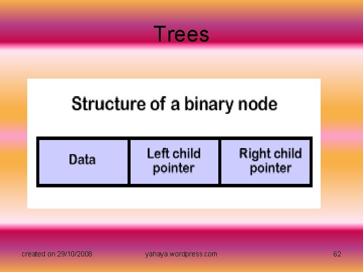
Trees • Now let's examine one way that trees are implemented in the computer's memory. We will begin by introducing a simple tree structure called a binary tree. Binary trees have the restriction that nodes can have no more than two children. With this restriction, we can easily determine how to represent a single binary node in memory. Our node will need to reserve memory for data and two pointers. created on 29/10/2008 yahaya. wordpress. com 61

Trees created on 29/10/2008 yahaya. wordpress. com 62

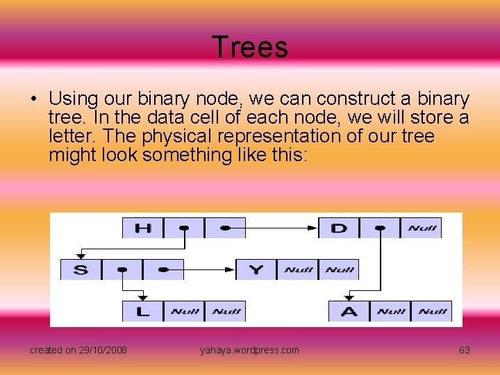
Trees • Using our binary node, we can construct a binary tree. In the data cell of each node, we will store a letter. The physical representation of our tree might look something like this: created on 29/10/2008 yahaya. wordpress. com 63

Trees • Although the diagram above represents a tree, it doesn't look much like the tree we examined from the XYZ company. Because our tree uses pointers, the physical representation is much different than the logical representation. Starting with the root node of the binary tree (the node that contains 'H'), see if you can draw a sketch of the logical representation of this tree. Once you are finished, you may view the answer. created on 29/10/2008 yahaya. wordpress. com 64

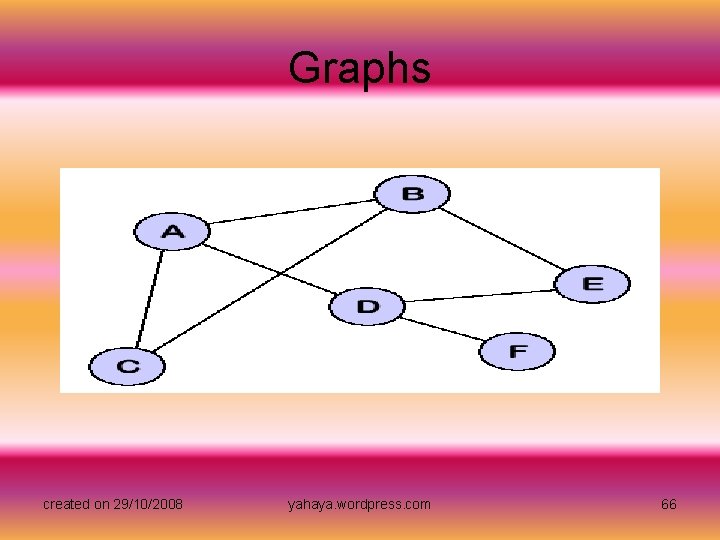
Graphs • The last data structure that we will study in this section is the graph. Graphs are similar to trees except they do not have as many restrictions. In the previous lesson, we saw that every tree has a root node, and all the other nodes in the tree are children of this node. We also saw that nodes can have many children but only one parent. When we relax these restrictions, we get the graph data structure. The logical representation of a typical graph might look something like this: created on 29/10/2008 yahaya. wordpress. com 65

Graphs created on 29/10/2008 yahaya. wordpress. com 66

Graphs • Notice that our graph does not have a root node like the tree data structure did. Instead, any node can be connected with any other node. Nodes do not have a clear parent/child relationship like we saw in the tree. Instead nodes are called neighbors if they are connected by an edge. For example, node A above has three neighbors: B, C, and D. • It is not hard to imagine how the graph data structure could be useful for representing data. Perhaps each of the nodes above could represent a city and the edges connecting the nodes could represent roads. Or we could use a graph to represent a computer network where the nodes are workstations and the edges are network connections. Graphs have so many applications in computer science and mathematics that several algorithms have been written to perform standard graph operations such as searching the graph and finding the shortest path between nodes of a graph. created on 29/10/2008 yahaya. wordpress. com 67

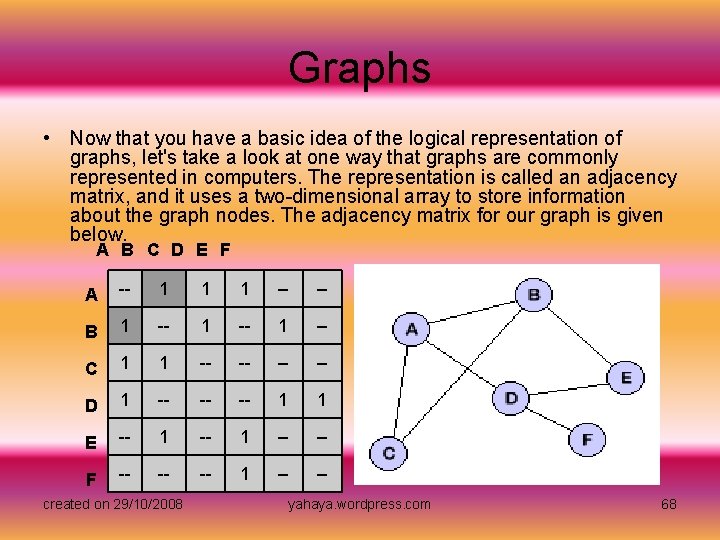
Graphs • Now that you have a basic idea of the logical representation of graphs, let's take a look at one way that graphs are commonly represented in computers. The representation is called an adjacency matrix, and it uses a two-dimensional array to store information about the graph nodes. The adjacency matrix for our graph is given below. A B C D E F A -- 1 1 1 -- -- B 1 -- C 1 1 -- -- D 1 -- -- -- 1 1 E -- 1 -- -- F -- -- -- 1 -- -- created on 29/10/2008 yahaya. wordpress. com 68

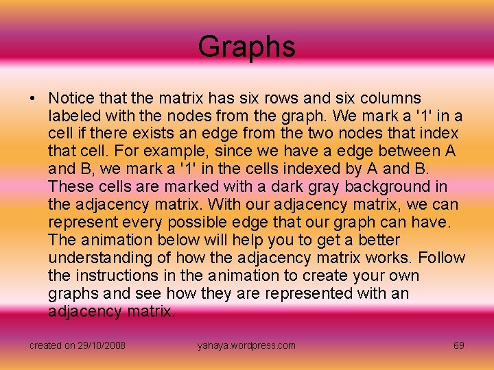
Graphs • Notice that the matrix has six rows and six columns labeled with the nodes from the graph. We mark a '1' in a cell if there exists an edge from the two nodes that index that cell. For example, since we have a edge between A and B, we mark a '1' in the cells indexed by A and B. These cells are marked with a dark gray background in the adjacency matrix. With our adjacency matrix, we can represent every possible edge that our graph can have. The animation below will help you to get a better understanding of how the adjacency matrix works. Follow the instructions in the animation to create your own graphs and see how they are represented with an adjacency matrix. created on 29/10/2008 yahaya. wordpress. com 69

Abstract Data Types • The concept of data structures is closely related to another important concept in computer science called abstract data types. Recall the definition of a data type: "a data type consists of the values it represents and the operations defined upon it. " You are already familiar with some basic data types such as integers and characters. These data types are found in nearly all computers, and they have well-defined operations that can be done with them. For example, the integer data type has operations for addition, subtraction, multiplication, and division. The computer knows how to perform these arithmetic operations with any two integers because these operations are part of the integer data type. created on 29/10/2008 yahaya. wordpress. com 70

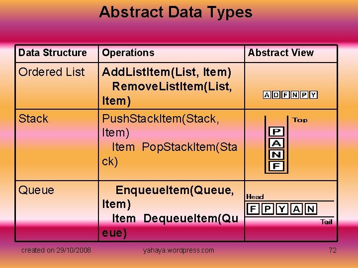
Abstract Data Types • We can extend the idea of data types to include more than just the basic data types. Our definition of data types consists of two parts: 1) values, and 2) operations. Now suppose we extended our definition so that the first part included data structures. This extension makes sense because our data structures are really just novel ways of organizing values. We have already seen several examples of these extended or abstract data types (ADTs). The examples that we studied are listed below. created on 29/10/2008 yahaya. wordpress. com 71

Abstract Data Types Data Structure Operations Ordered List Add. List. Item(List, Item) Remove. List. Item(List, Item) Stack Push. Stack. Item(Stack, Item) Item Pop. Stack. Item(Sta ck) Queue Enqueue. Item(Queue, Item) Item Dequeue. Item(Qu eue) created on 29/10/2008 yahaya. wordpress. com Abstract View 72

Abstract Data Types • Notice that each of the ADTs above has the two elements required by our definition: 1) a particular data structure, and 2) operations related to the data structure. We call these data types "abstract" because we have said nothing about how they are implemented. Instead, we have defined an interface for using the data type which consists of certain operations. The interface for an ADT remains the same regardless of how the data structure and operations are implemented. For example, we can use the stack ADT in a computer program by using the two operations defined in the stack interface. We do not need to know whether these operations were implemented using a linked list or an array. created on 29/10/2008 yahaya. wordpress. com 73

Abstract Data Types • Now let's consider how to create a new ADT using our definition. First, we must choose a particular data structure. Remember that data structures are simply ways of organizing data in the computer. For our ADT, we will use a bag data structure. This structure is based on the idea of storing various items into a bag just as you might put various groceries in a grocery bag. We want our data structure to have the same properties that real bags have. • Second, we need to define an interface for our ADT by specifying the operations it will support. Since we are modeling a bag, we will choose operations that give our data structure the same functionality that a grocery bag might have. The applet below shows the interface for our data structure as a row of buttons. Try each of the operations to discover how the bag ADT works. You will be asked to describe these operations in the review questions. created on 29/10/2008 yahaya. wordpress. com 74

Summary of Data Structures • Let's take a quick review of all that we have learned about data structures in these lessons. 1. We began by introducing the idea of a data structure as a way of organizing data in a computer's memory. We discussed how a computer's memory is organized as a long row of memory cells with each cell having a particular address. We also examined how these memory cells can contain the address of another memory cell. These pointers allow us to build very flexible and complex data structures. created on 29/10/2008 yahaya. wordpress. com 75

Summary of Data Structures 2. We examined a class of data structures called linear data structures that are organized in a linear fashion similar to the computer's memory. The first linear data structure was the ordered list. With this data structure we introduced the idea of abstraction and implementation. We saw there are two different ways to implement a list, but both implementations still have the same list operations. The second linear data structure was the stack. We discovered that the stack is really a list with the restriction that items can only be added and removed from the top of the stack. The third linear data structure was the queue. As we studied the queue, we found that our queue implementation had two distinct representations: logical and physical. In the logical representation, our queue was similar to a ring, but in the physical representation, our queue was actually implemented with an array. created on 29/10/2008 yahaya. wordpress. com 76

Summary of Data Structures 3. We looked at another class of data structures call nonlinear data structures that are organized quite differently from the computer's memory. These data structures included multidimensional arrays, trees, and graphs. For each data structure, we examined one implementation of the data structure and discussed how the logical representation of the data structure was different from the physical representation. 4. We introduced the idea of an abstract data type that groups a data structure with certain operations. These operations form an interface for the ADT through which the data structure can be manipulated. created on 29/10/2008 yahaya. wordpress. com 77