Lesson 9 Confidence Intervals and Tests of Hypothesis

Lesson 9: Confidence Intervals and Tests of Hypothesis Two or more samples Ka-fu Wong © 2007 ECON 1003: Analysis of Economic Data Lesson 9 -1

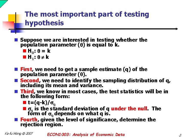
The most important part of testing hypothesis n Suppose we are interested in testing whether the population parameter ( ) is equal to k. n H 0: = k n H 1: k n First, we need to get a sample estimate (q) of the population parameter ( ). n Second, we need to identify the sampling distribution of q, including its mean and variance. n Third, we know in most cases, the test statistics will be in the following form: n t=(q-k)/ q n q is the standard deviation of q under the null. The form of q depends on what q is. n Fourth, given the level of significance, determine the rejection region. Ka-fu Wong © 2007 ECON 1003: Analysis of Economic Data 2

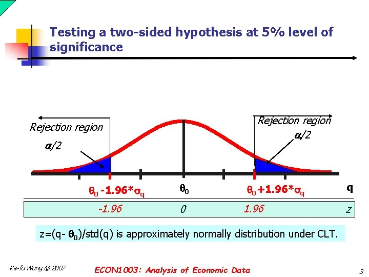
Testing a two-sided hypothesis at 5% level of significance Rejection region /2 0 -1. 96* q -1. 96 0 0 0+1. 96* q 1. 96 q z z=(q- 0)/std(q) is approximately normally distribution under CLT. Ka-fu Wong © 2007 ECON 1003: Analysis of Economic Data 3

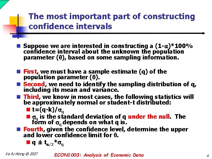
The most important part of constructing confidence intervals n Suppose we are interested in constructing a (1 - )*100% confidence interval about the unknown the population parameter ( ), based on some sampling information. n First, we must have a sample estimate (q) of the population parameter ( ). n Second, we need to identify the sampling distribution of q, including its mean and variance. n Third, we know in most cases, the following statistics will be approximately normal or student-t distributed: n t=(q-k)/ q n q is the standard deviation of q under the null. The form of q depends on what q is. n Fourth, given the confidence level, determine the upper and lower confidence limit for . n q ± t /2* q Ka-fu Wong © 2007 ECON 1003: Analysis of Economic Data 4

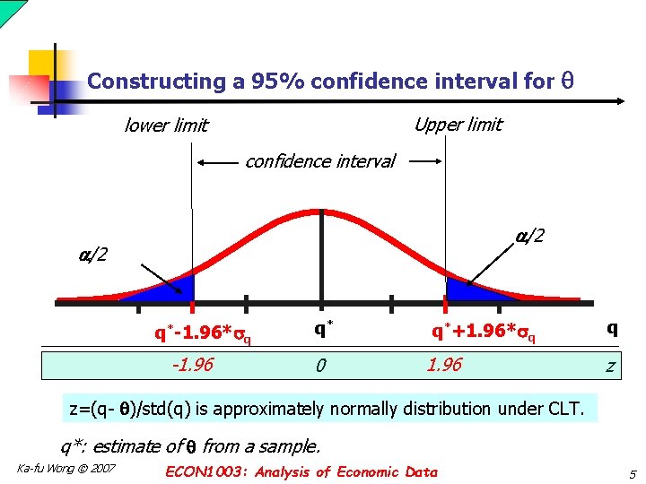
Constructing a 95% confidence interval for Upper limit lower limit confidence interval /2 q*-1. 96* q -1. 96 q* 0 q*+1. 96* q 1. 96 q z z=(q- )/std(q) is approximately normally distribution under CLT. q*: estimate of from a sample. Ka-fu Wong © 2007 ECON 1003: Analysis of Economic Data 5

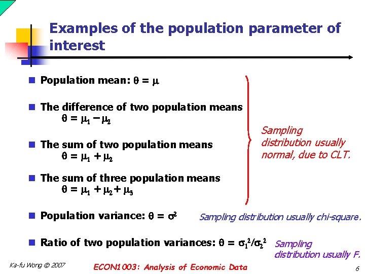
Examples of the population parameter of interest n Population mean: = m n The difference of two population means = m 1 – m 2 n The sum of two population means = m 1 + m 2 Sampling distribution usually normal, due to CLT. n The sum of three population means = m 1 + m 2 + m 3 n Population variance: = 2 Sampling distribution usually chi-square. n Ratio of two population variances: = 12/ 22 Sampling distribution usually F. Ka-fu Wong © 2007 ECON 1003: Analysis of Economic Data 6

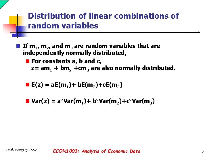
Distribution of linear combinations of random variables n If m 1, m 2, and m 3 are random variables that are independently normally distributed, n For constants a, b and c, z= am 1 + bm 2 +cm 3 are also normally distributed. n E(z) = a. E(m 1)+ b. E(m 2)+c. E(m 3) n Var(z) = a 2 Var(m 1)+ b 2 Var(m 2)+c 2 Var(m 3) Ka-fu Wong © 2007 ECON 1003: Analysis of Economic Data 7

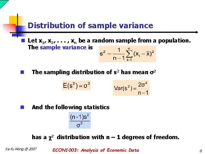
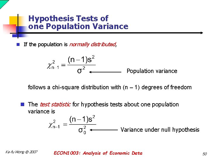
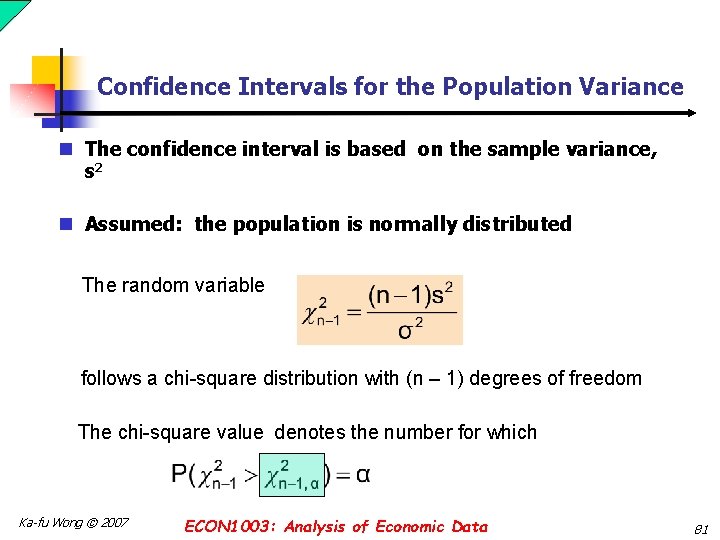
Distribution of sample variance n Let x 1, x 2, . . . , xn be a random sample from a population. The sample variance is n The sampling distribution of s 2 has mean σ2 n And the following statistics has a 2 distribution with n – 1 degrees of freedom. Ka-fu Wong © 2007 ECON 1003: Analysis of Economic Data 8

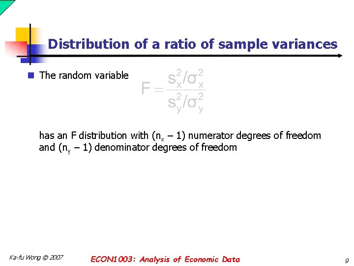
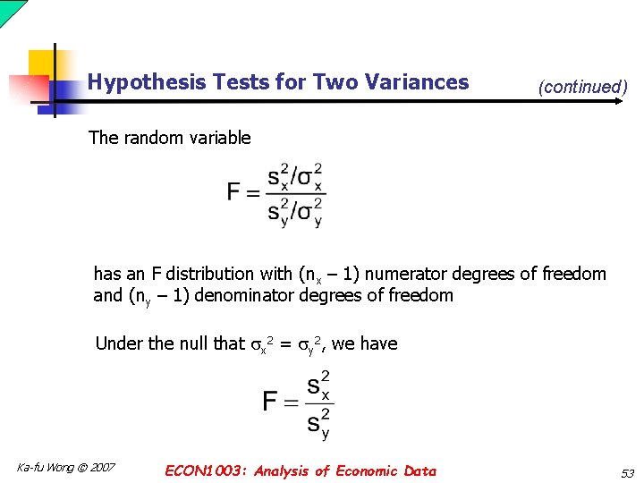
Distribution of a ratio of sample variances n The random variable has an F distribution with (nx – 1) numerator degrees of freedom and (ny – 1) denominator degrees of freedom Ka-fu Wong © 2007 ECON 1003: Analysis of Economic Data 9

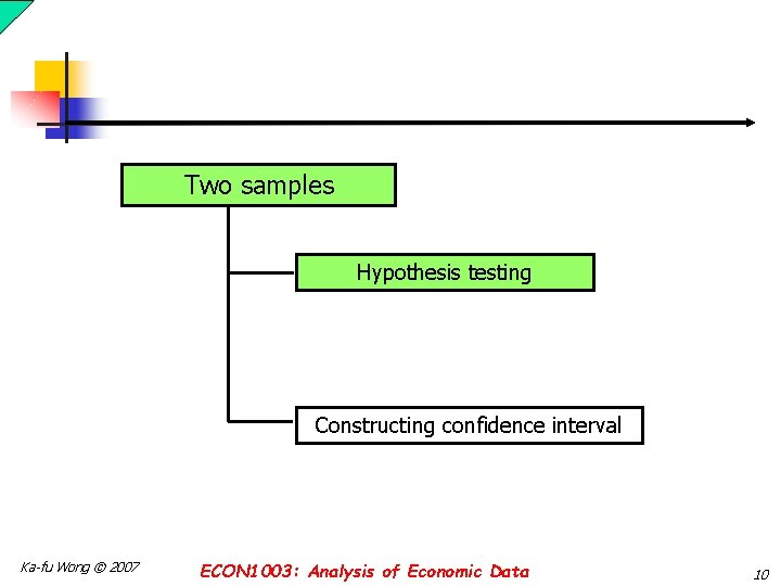
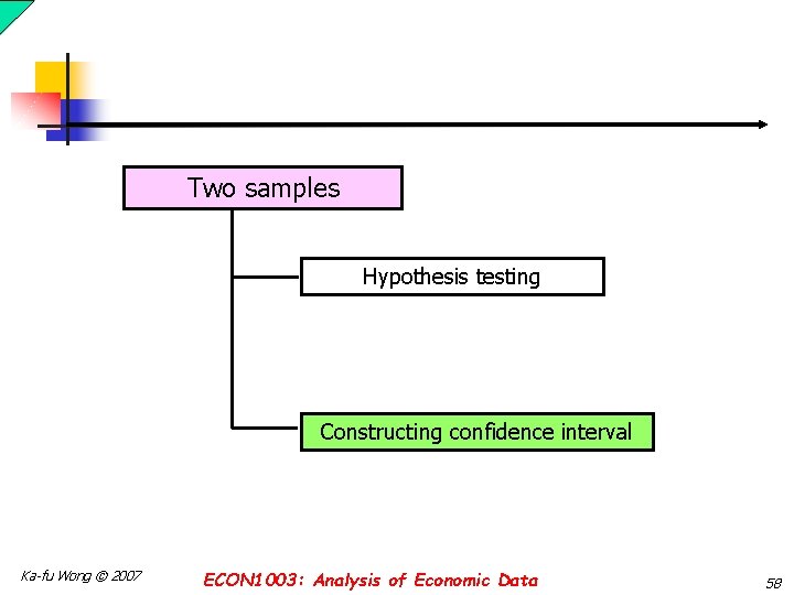
Two samples Hypothesis testing Constructing confidence interval Ka-fu Wong © 2007 ECON 1003: Analysis of Economic Data 10

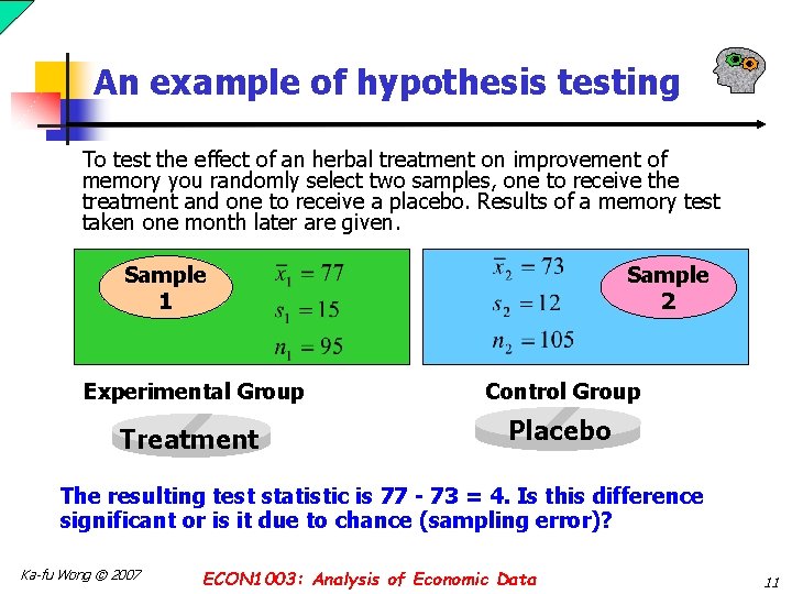
An example of hypothesis testing To test the effect of an herbal treatment on improvement of memory you randomly select two samples, one to receive the treatment and one to receive a placebo. Results of a memory test taken one month later are given. Sample 1 Sample 2 Experimental Group Control Group Treatment Placebo The resulting test statistic is 77 - 73 = 4. Is this difference significant or is it due to chance (sampling error)? Ka-fu Wong © 2007 ECON 1003: Analysis of Economic Data 11

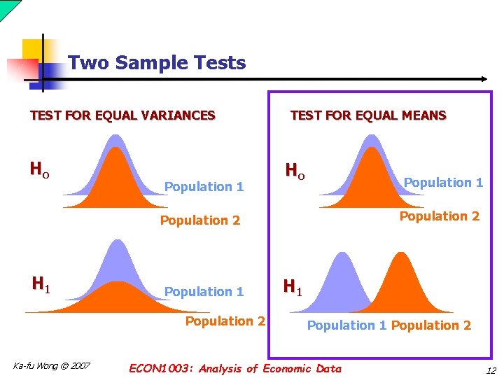
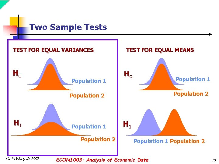
Two Sample Tests TEST FOR EQUAL VARIANCES Ho Population 1 TEST FOR EQUAL MEANS Ho Population 1 Population 2 H 1 Population 2 Ka-fu Wong © 2007 H 1 Population 2 ECON 1003: Analysis of Economic Data 12

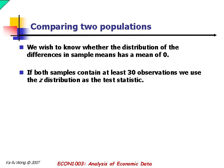
Comparing two populations n We wish to know whether the distribution of the differences in sample means has a mean of 0. n If both samples contain at least 30 observations we use the z distribution as the test statistic. Ka-fu Wong © 2007 ECON 1003: Analysis of Economic Data

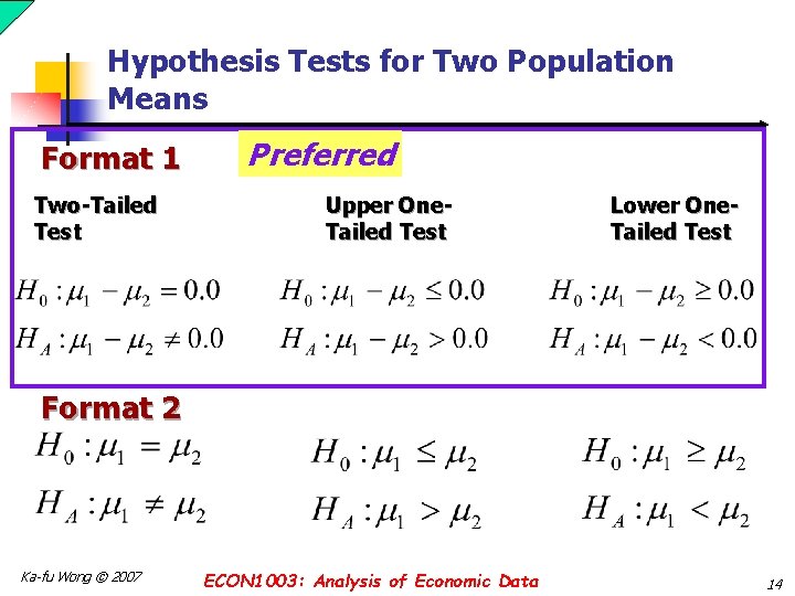
Hypothesis Tests for Two Population Means Format 1 Two-Tailed Test Preferred Upper One. Tailed Test Lower One. Tailed Test Format 2 Ka-fu Wong © 2007 ECON 1003: Analysis of Economic Data 14

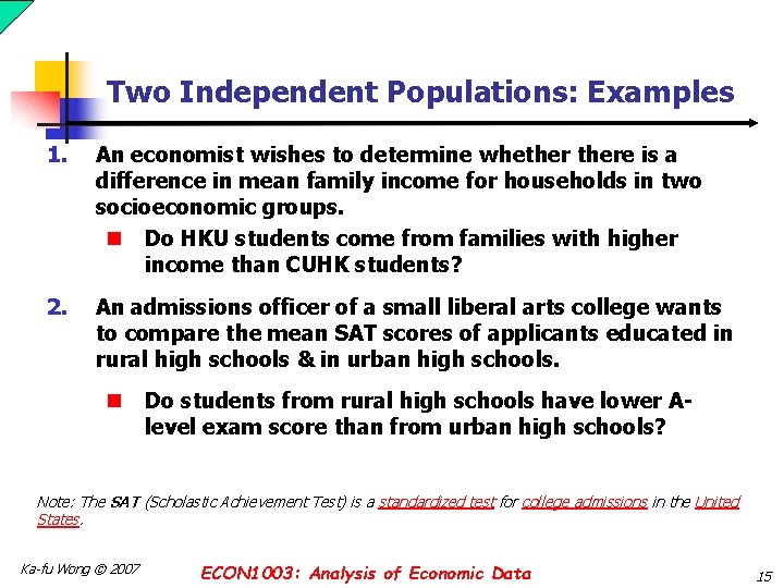
Two Independent Populations: Examples 1. An economist wishes to determine whethere is a difference in mean family income for households in two socioeconomic groups. n Do HKU students come from families with higher income than CUHK students? 2. An admissions officer of a small liberal arts college wants to compare the mean SAT scores of applicants educated in rural high schools & in urban high schools. n Do students from rural high schools have lower Alevel exam score than from urban high schools? Note: The SAT (Scholastic Achievement Test) is a standardized test for college admissions in the United States. Ka-fu Wong © 2007 ECON 1003: Analysis of Economic Data 15

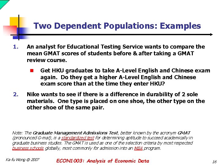
Two Dependent Populations: Examples 1. An analyst for Educational Testing Service wants to compare the mean GMAT scores of students before & after taking a GMAT review course. n 2. Get HKU graduates to take A-Level English and Chinese exam again. Do they get a higher A-Level English and Chinese exam score than at the time they enter HKU? Nike wants to see if there is a difference in durability of 2 sole materials. One type is placed on one shoe, the other type on the other shoe of the same pair. Note: The Graduate Management Admissions Test, better known by the acronym GMAT (pronounced G-mat), is a standardized test for determining aptitude to succeed academically in graduate business studies. The GMAT is used as one of the selection criteria by most respected business schools globally, most commonly for admission into an MBA program. Ka-fu Wong © 2007 ECON 1003: Analysis of Economic Data 16

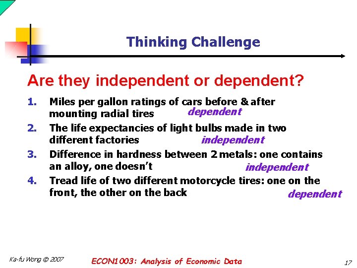
Thinking Challenge Are they independent or dependent? 1. 2. 3. 4. Miles per gallon ratings of cars before & after dependent mounting radial tires The life expectancies of light bulbs made in two different factories independent Difference in hardness between 2 metals: one contains an alloy, one doesn’t independent Tread life of two different motorcycle tires: one on the front, the other on the back dependent Ka-fu Wong © 2007 ECON 1003: Analysis of Economic Data 17

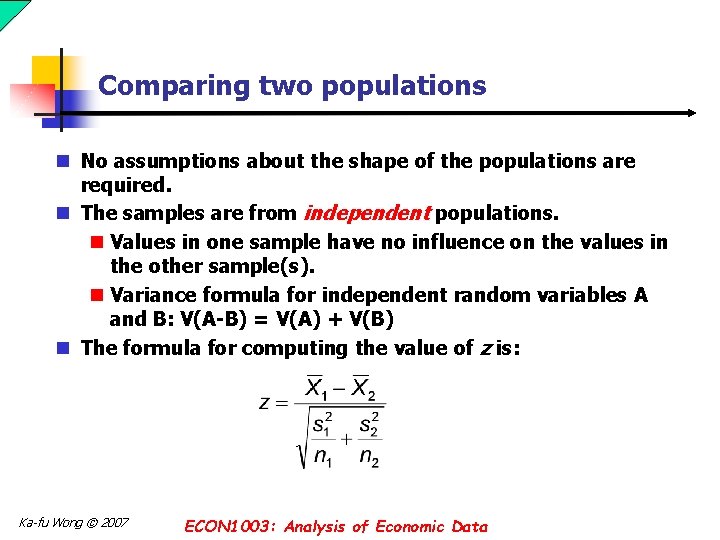
Comparing two populations n No assumptions about the shape of the populations are required. n The samples are from independent populations. n Values in one sample have no influence on the values in the other sample(s). n Variance formula for independent random variables A and B: V(A-B) = V(A) + V(B) n The formula for computing the value of z is: Ka-fu Wong © 2007 ECON 1003: Analysis of Economic Data

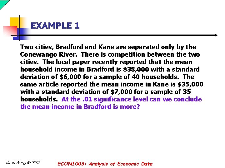
EXAMPLE 1 Two cities, Bradford and Kane are separated only by the Conewango River. There is competition between the two cities. The local paper recently reported that the mean household income in Bradford is $38, 000 with a standard deviation of $6, 000 for a sample of 40 households. The same article reported the mean income in Kane is $35, 000 with a standard deviation of $7, 000 for a sample of 35 households. At the. 01 significance level can we conclude the mean income in Bradford is more? Ka-fu Wong © 2007 ECON 1003: Analysis of Economic Data

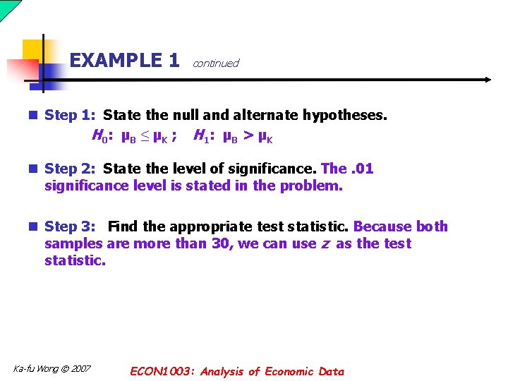
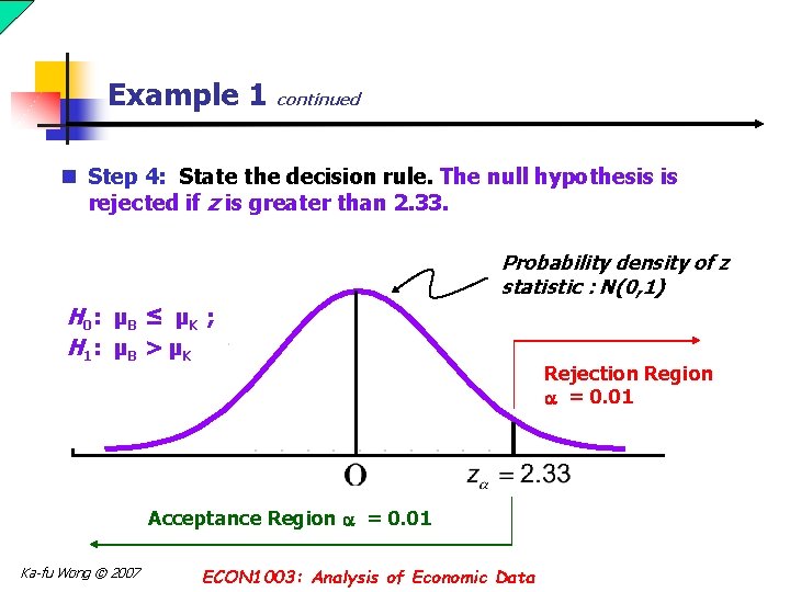
EXAMPLE 1 continued n Step 1: State the null and alternate hypotheses. H 0: µB ≤ µK ; H 1: µB > µK n Step 2: State the level of significance. The. 01 significance level is stated in the problem. n Step 3: Find the appropriate test statistic. Because both samples are more than 30, we can use z as the test statistic. Ka-fu Wong © 2007 ECON 1003: Analysis of Economic Data

Example 1 continued n Step 4: State the decision rule. The null hypothesis is rejected if z is greater than 2. 33. Probability density of z statistic : N(0, 1) H 0: µB ≤ µK ; H 1: µB > µK Acceptance Region = 0. 01 Ka-fu Wong © 2007 ECON 1003: Analysis of Economic Data Rejection Region = 0. 01

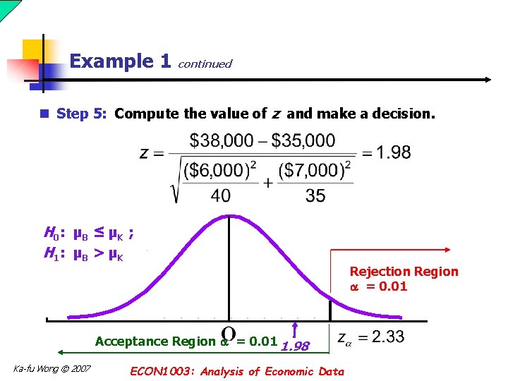
Example 1 continued n Step 5: Compute the value of z and make a decision. H 0: µB ≤ µK ; H 1: µB > µK Acceptance Region = 0. 01 1. 98 Ka-fu Wong © 2007 ECON 1003: Analysis of Economic Data Rejection Region = 0. 01

Example 1 continued n The decision is to not reject the null hypothesis. We cannot conclude that the mean household income in Bradford is larger. Ka-fu Wong © 2007 ECON 1003: Analysis of Economic Data

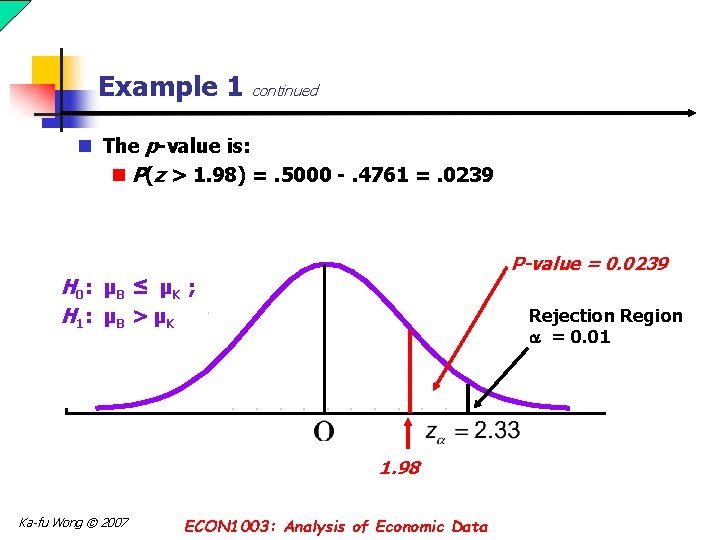
Example 1 continued n The p-value is: n P(z > 1. 98) =. 5000 -. 4761 =. 0239 P-value = 0. 0239 H 0: µB ≤ µK ; H 1: µB > µK Rejection Region = 0. 01 1. 98 Ka-fu Wong © 2007 ECON 1003: Analysis of Economic Data

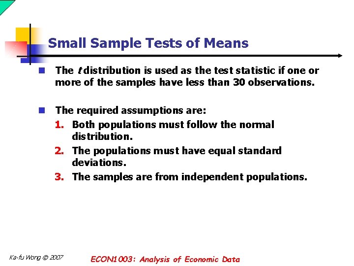
Small Sample Tests of Means n The t distribution is used as the test statistic if one or more of the samples have less than 30 observations. n The required assumptions are: 1. Both populations must follow the normal distribution. 2. The populations must have equal standard deviations. 3. The samples are from independent populations. Ka-fu Wong © 2007 ECON 1003: Analysis of Economic Data

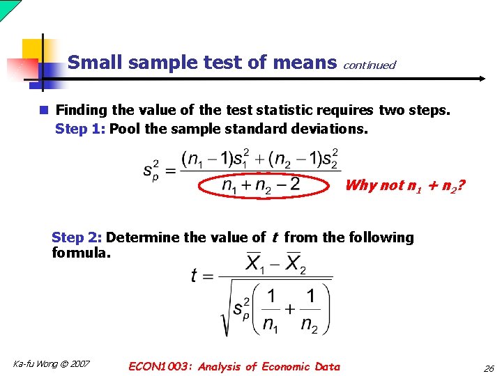
Small sample test of means continued n Finding the value of the test statistic requires two steps. Step 1: Pool the sample standard deviations. Why not n 1 + n 2? Step 2: Determine the value of t from the following formula. Ka-fu Wong © 2007 ECON 1003: Analysis of Economic Data 26

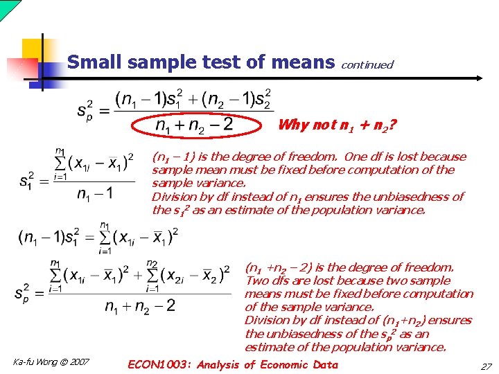
Small sample test of means continued Why not n 1 + n 2? (n 1 – 1) is the degree of freedom. One df is lost because sample mean must be fixed before computation of the sample variance. Division by df instead of n 1 ensures the unbiasedness of the s 12 as an estimate of the population variance. (n 1 +n 2 – 2) is the degree of freedom. Two dfs are lost because two sample means must be fixed before computation of the sample variance. Division by df instead of (n 1+n 2) ensures the unbiasedness of the sp 2 as an estimate of the population variance. Ka-fu Wong © 2007 ECON 1003: Analysis of Economic Data 27

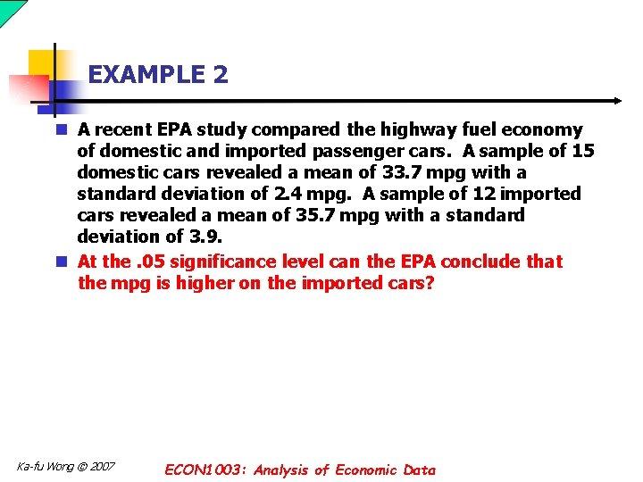
EXAMPLE 2 n A recent EPA study compared the highway fuel economy of domestic and imported passenger cars. A sample of 15 domestic cars revealed a mean of 33. 7 mpg with a standard deviation of 2. 4 mpg. A sample of 12 imported cars revealed a mean of 35. 7 mpg with a standard deviation of 3. 9. n At the. 05 significance level can the EPA conclude that the mpg is higher on the imported cars? Ka-fu Wong © 2007 ECON 1003: Analysis of Economic Data

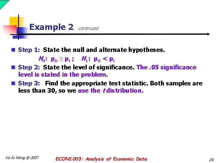
Example 2 continued n Step 1: State the null and alternate hypotheses. H 0: µD ≥ µI ; H 1: µD < µI n Step 2: State the level of significance. The. 05 significance level is stated in the problem. n Step 3: Find the appropriate test statistic. Both samples are less than 30, so we use the t distribution. Ka-fu Wong © 2007 ECON 1003: Analysis of Economic Data 29

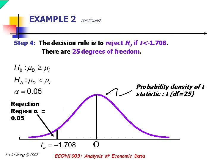
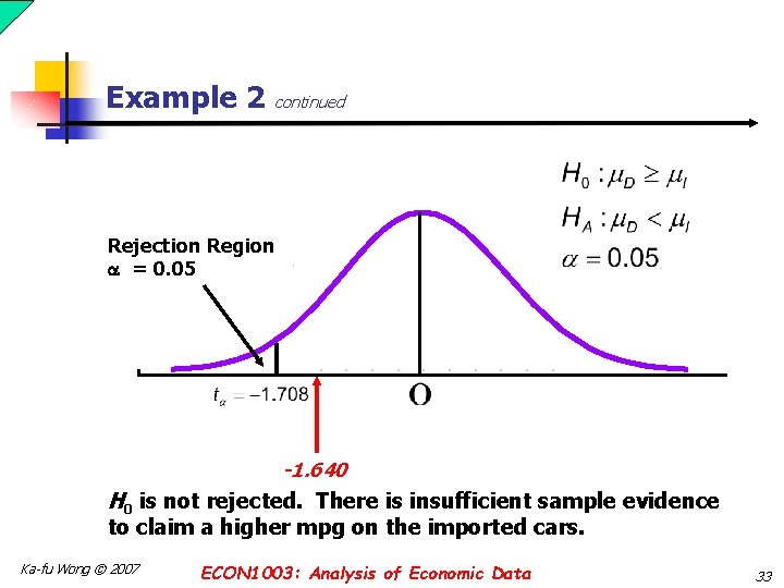
EXAMPLE 2 continued Step 4: The decision rule is to reject H 0 if t<-1. 708. There are 25 degrees of freedom. Probability density of t statistic : t (df=25) Rejection Region = 0. 05 Ka-fu Wong © 2007 ECON 1003: Analysis of Economic Data

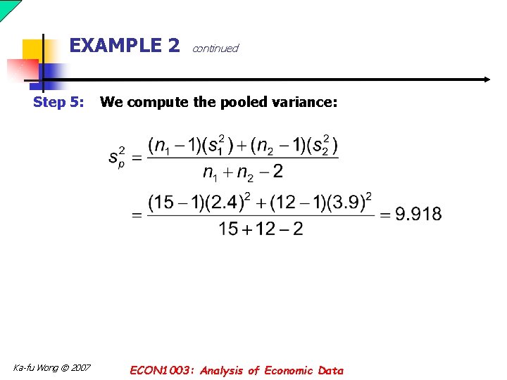
EXAMPLE 2 Step 5: Ka-fu Wong © 2007 continued We compute the pooled variance: ECON 1003: Analysis of Economic Data

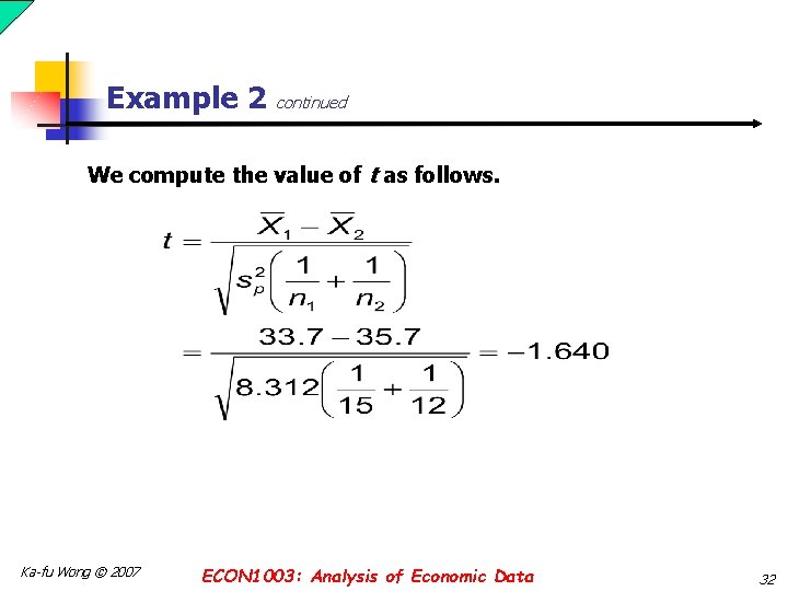
Example 2 continued We compute the value of t as follows. Ka-fu Wong © 2007 ECON 1003: Analysis of Economic Data 32

Example 2 continued Rejection Region = 0. 05 -1. 640 H 0 is not rejected. There is insufficient sample evidence to claim a higher mpg on the imported cars. Ka-fu Wong © 2007 ECON 1003: Analysis of Economic Data 33

Hypothesis Testing Involving Paired Observations n Independent samples are samples that are not related in any way. n Dependent samples are samples that are paired or related in some fashion. For example: n If you wished to buy a car you would look at the same car at two (or more) different dealerships and compare the prices. n If you wished to measure the effectiveness of a new diet you would weigh the dieters at the start and at the finish of the program. Ka-fu Wong © 2007 ECON 1003: Analysis of Economic Data

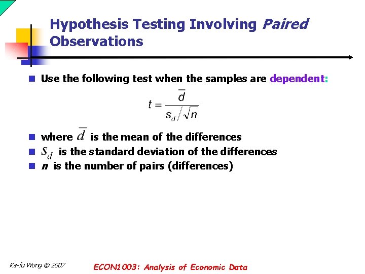
Hypothesis Testing Involving Paired Observations n Use the following test when the samples are dependent: n where is the mean of the differences n is the standard deviation of the differences n n is the number of pairs (differences) Ka-fu Wong © 2007 ECON 1003: Analysis of Economic Data

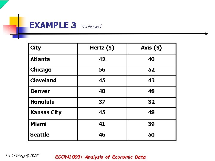
EXAMPLE 3 n An independent testing agency is comparing the daily rental cost for renting a compact car from Hertz and Avis. A random sample of eight cities revealed the following information. At the. 05 significance level can the testing agency conclude that there is a difference in the rental charged? Ka-fu Wong © 2007 ECON 1003: Analysis of Economic Data

EXAMPLE 3 City continued Hertz ($) Avis ($) Atlanta 42 40 Chicago 56 52 Cleveland 45 43 Denver 48 48 Honolulu 37 32 Kansas City 45 48 Miami 41 39 Seattle 46 50 Ka-fu Wong © 2007 ECON 1003: Analysis of Economic Data

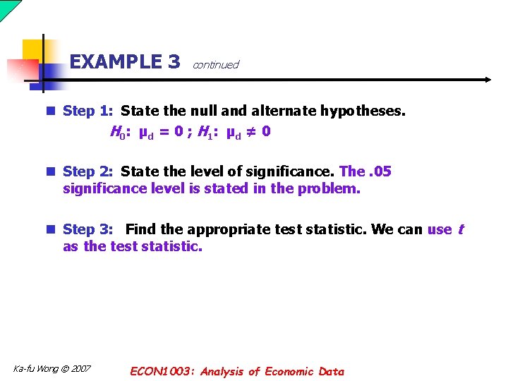
EXAMPLE 3 continued n Step 1: State the null and alternate hypotheses. H 0: µd = 0 ; H 1: µd ≠ 0 n Step 2: State the level of significance. The. 05 significance level is stated in the problem. n Step 3: Find the appropriate test statistic. We can use t as the test statistic. Ka-fu Wong © 2007 ECON 1003: Analysis of Economic Data

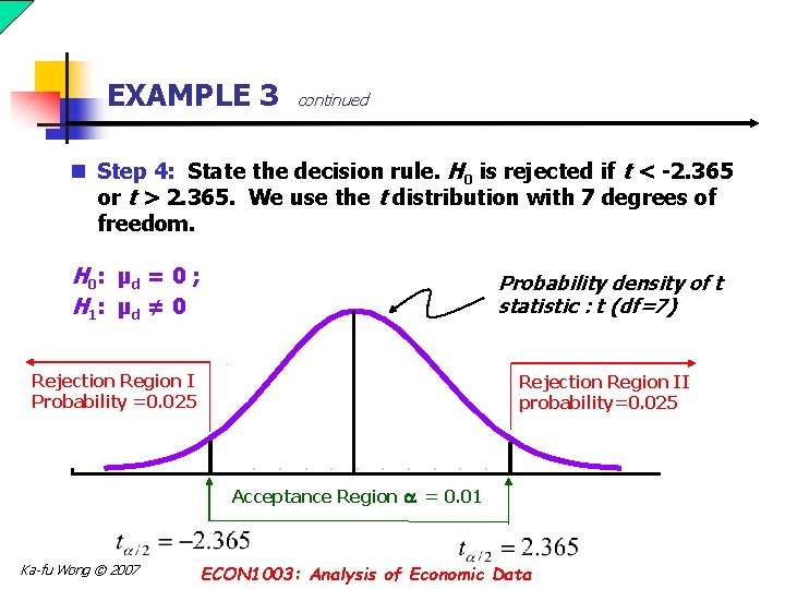
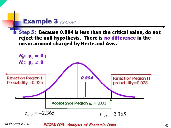
EXAMPLE 3 continued n Step 4: State the decision rule. H 0 is rejected if t < -2. 365 or t > 2. 365. We use the t distribution with 7 degrees of freedom. H 0: µd = 0 ; H 1: µd ≠ 0 Probability density of t statistic : t (df=7) Rejection Region I Probability =0. 025 Rejection Region II probability=0. 025 Acceptance Region = 0. 01 Ka-fu Wong © 2007 ECON 1003: Analysis of Economic Data

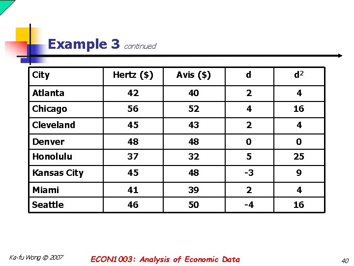
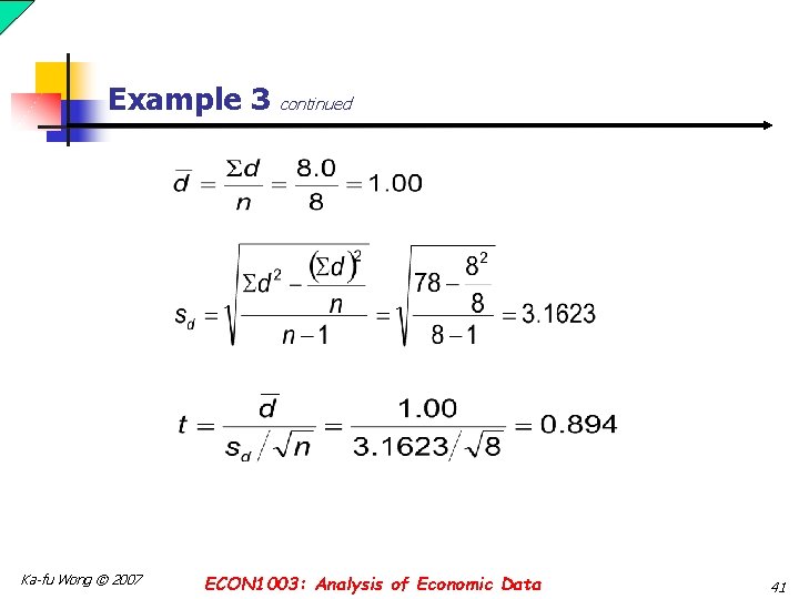
Example 3 continued City Hertz ($) Avis ($) d d 2 Atlanta 42 40 2 4 Chicago 56 52 4 16 Cleveland 45 43 2 4 Denver 48 48 0 0 Honolulu 37 32 5 25 Kansas City 45 48 -3 9 Miami 41 39 2 4 Seattle 46 50 -4 16 Ka-fu Wong © 2007 ECON 1003: Analysis of Economic Data 40

Example 3 continued Ka-fu Wong © 2007 ECON 1003: Analysis of Economic Data 41

Example 3 continued n Step 5: Because 0. 894 is less than the critical value, do not reject the null hypothesis. There is no difference in the mean amount charged by Hertz and Avis. H 0: µd = 0 ; H 1: µd ≠ 0 Rejection Region I Probability =0. 025 0. 894 Rejection Region II probability=0. 025 Acceptance Region = 0. 01 Ka-fu Wong © 2007 ECON 1003: Analysis of Economic Data 42

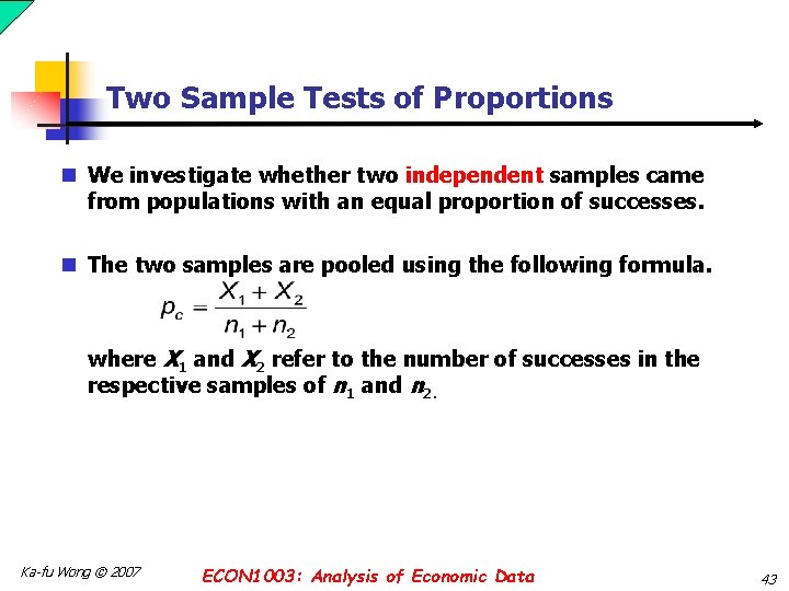
Two Sample Tests of Proportions n We investigate whether two independent samples came from populations with an equal proportion of successes. n The two samples are pooled using the following formula. where X 1 and X 2 refer to the number of successes in the respective samples of n 1 and n 2. Ka-fu Wong © 2007 ECON 1003: Analysis of Economic Data 43

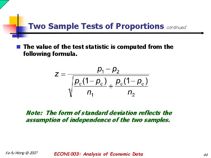
Two Sample Tests of Proportions continued n The value of the test statistic is computed from the following formula. Note: The form of standard deviation reflects the assumption of independence of the two samples. Ka-fu Wong © 2007 ECON 1003: Analysis of Economic Data 44

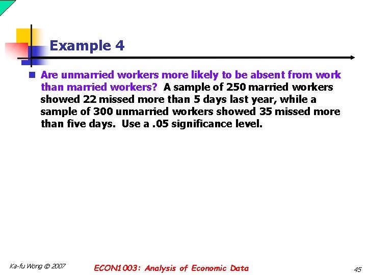
Example 4 n Are unmarried workers more likely to be absent from work than married workers? A sample of 250 married workers showed 22 missed more than 5 days last year, while a sample of 300 unmarried workers showed 35 missed more than five days. Use a. 05 significance level. Ka-fu Wong © 2007 ECON 1003: Analysis of Economic Data 45

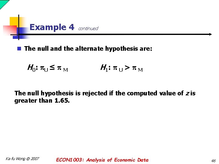
Example 4 continued n The null and the alternate hypothesis are: H 0 : U ≤ M H 1 : U > M The null hypothesis is rejected if the computed value of z is greater than 1. 65. Ka-fu Wong © 2007 ECON 1003: Analysis of Economic Data 46

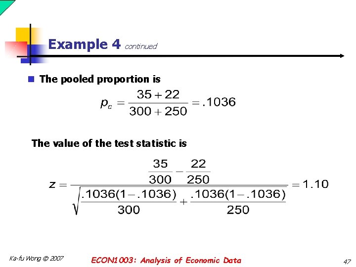
Example 4 continued n The pooled proportion is The value of the test statistic is Ka-fu Wong © 2007 ECON 1003: Analysis of Economic Data 47

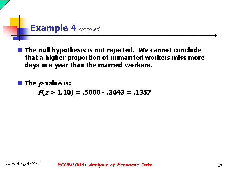
Example 4 continued n The null hypothesis is not rejected. We cannot conclude that a higher proportion of unmarried workers miss more days in a year than the married workers. n The p-value is: P(z > 1. 10) =. 5000 -. 3643 =. 1357 Ka-fu Wong © 2007 ECON 1003: Analysis of Economic Data 48

Two Sample Tests TEST FOR EQUAL VARIANCES Ho Population 1 TEST FOR EQUAL MEANS Ho Population 1 Population 2 H 1 Population 2 Ka-fu Wong © 2007 H 1 Population 2 ECON 1003: Analysis of Economic Data 49

Hypothesis Tests of one Population Variance n If the population is normally distributed, Population variance follows a chi-square distribution with (n – 1) degrees of freedom n The test statistic for hypothesis tests about one population variance is Variance under null hypothesis Ka-fu Wong © 2007 ECON 1003: Analysis of Economic Data 50

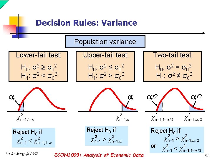
Decision Rules: Variance Population variance Lower-tail test: Upper-tail test: Two-tail test: H 0: σ 2 σ 02 H 1: σ 2 < σ 02 H 0: σ 2 ≤ σ 02 H 1: σ 2 > σ 02 H 0: σ 2 = σ 02 H 1: σ 2 ≠ σ 02 Reject H 0 if /2 Reject H 0 if or Ka-fu Wong © 2007 ECON 1003: Analysis of Economic Data 51

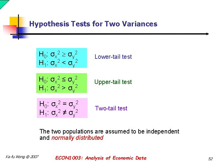
Hypothesis Tests for Two Variances H 0: σx 2 σy 2 H 1: σx 2 < σy 2 Lower-tail test H 0: σx 2 ≤ σy 2 H 1: σx 2 > σy 2 Upper-tail test H 0: σx 2 = σy 2 H 1: σx 2 ≠ σy 2 Two-tail test The two populations are assumed to be independent and normally distributed Ka-fu Wong © 2007 ECON 1003: Analysis of Economic Data 52

Hypothesis Tests for Two Variances (continued) The random variable has an F distribution with (nx – 1) numerator degrees of freedom and (ny – 1) denominator degrees of freedom Under the null that sx 2 = sy 2, we have Ka-fu Wong © 2007 ECON 1003: Analysis of Economic Data 53

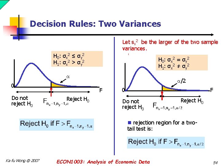
Decision Rules: Two Variances Let sx 2 be the larger of the two sample variances. H 0: σx 2 ≤ σy 2 H 1: σx 2 > σy 2 H 0: σx 2 = σy 2 H 1: σx 2 ≠ σy 2 0 Do not reject H 0 /2 F Reject H 0 0 F Do not reject H 0 Reject H 0 n rejection region for a twotail test is: Ka-fu Wong © 2007 ECON 1003: Analysis of Economic Data 54

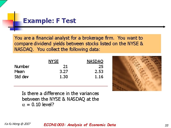
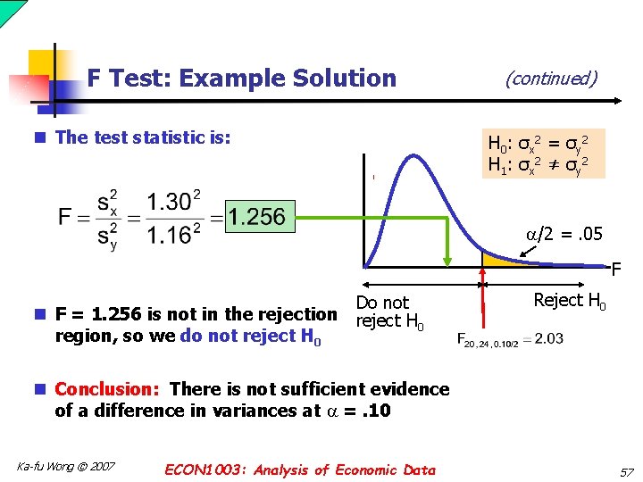
Example: F Test You are a financial analyst for a brokerage firm. You want to compare dividend yields between stocks listed on the NYSE & NASDAQ. You collect the following data: Number Mean Std dev NYSE 21 3. 27 1. 30 NASDAQ 25 2. 53 1. 16 Is there a difference in the variances between the NYSE & NASDAQ at the = 0. 10 level? Ka-fu Wong © 2007 ECON 1003: Analysis of Economic Data 55

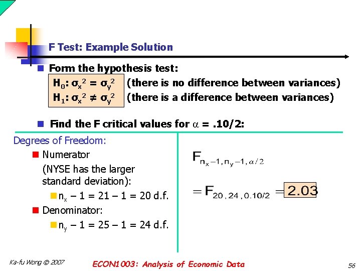
F Test: Example Solution n Form the hypothesis test: H 0: σx 2 = σy 2 (there is no difference between variances) H 1: σx 2 ≠ σy 2 (there is a difference between variances) n Find the F critical values for =. 10/2: Degrees of Freedom: n Numerator (NYSE has the larger standard deviation): n nx – 1 = 21 – 1 = 20 d. f. n Denominator: n ny – 1 = 25 – 1 = 24 d. f. Ka-fu Wong © 2007 ECON 1003: Analysis of Economic Data 56

F Test: Example Solution n The test statistic is: (continued) H 0: σx 2 = σy 2 H 1: σx 2 ≠ σy 2 /2 =. 05 F Do not n F = 1. 256 is not in the rejection reject H 0 region, so we do not reject H 0 Reject H 0 n Conclusion: There is not sufficient evidence of a difference in variances at =. 10 Ka-fu Wong © 2007 ECON 1003: Analysis of Economic Data 57

Two samples Hypothesis testing Constructing confidence interval Ka-fu Wong © 2007 ECON 1003: Analysis of Economic Data 58

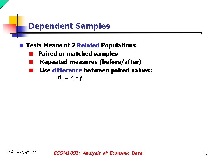
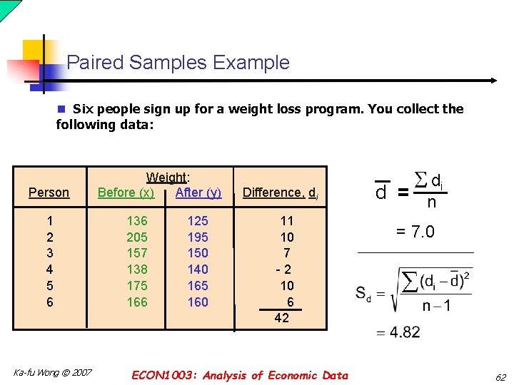
Dependent Samples n Tests Means of 2 Related Populations n Paired or matched samples n Repeated measures (before/after) n Use difference between paired values: d i = x i - yi Ka-fu Wong © 2007 ECON 1003: Analysis of Economic Data 59

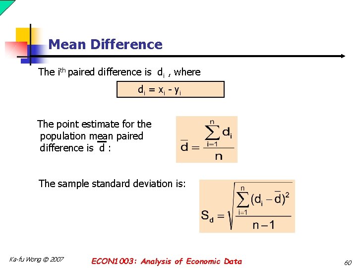
Mean Difference The ith paired difference is di , where d i = x i - yi The point estimate for the population mean paired difference is d : The sample standard deviation is: Ka-fu Wong © 2007 ECON 1003: Analysis of Economic Data 60

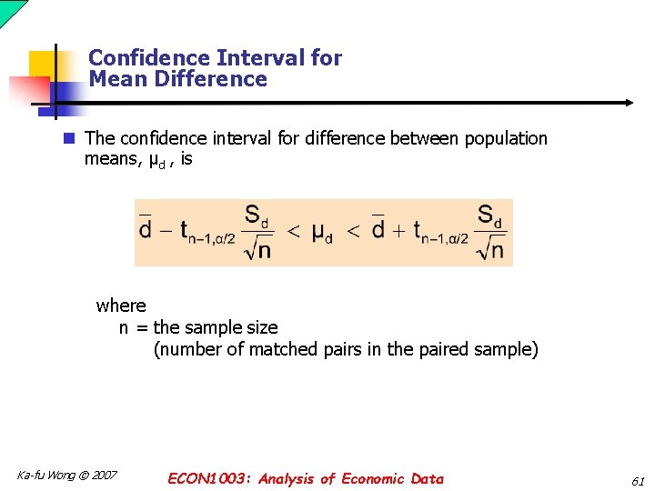
Confidence Interval for Mean Difference n The confidence interval for difference between population means, μd , is where n = the sample size (number of matched pairs in the paired sample) Ka-fu Wong © 2007 ECON 1003: Analysis of Economic Data 61

Paired Samples Example n Six people sign up for a weight loss program. You collect the following data: Person 1 2 3 4 5 6 Ka-fu Wong © 2007 Weight: Before (x) After (y) 136 205 157 138 175 166 125 195 150 140 165 160 Difference, di 11 10 7 -2 10 6 42 ECON 1003: Analysis of Economic Data di d = n = 7. 0 62

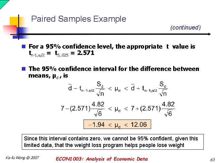
Paired Samples Example (continued) n For a 95% confidence level, the appropriate t value is tn-1, /2 = t 5, . 025 = 2. 571 n The 95% confidence interval for the difference between means, μd , is Since this interval contains zero, we cannot be 95% confident, given this limited data, that the weight loss program helps people lose weight Ka-fu Wong © 2007 ECON 1003: Analysis of Economic Data 63

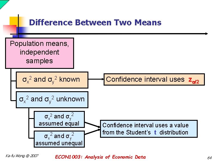
Difference Between Two Means Population means, independent samples σx 2 and σy 2 known Confidence interval uses z /2 σx 2 and σy 2 unknown σx 2 and σy 2 assumed equal σx 2 and σy 2 assumed unequal Ka-fu Wong © 2007 Confidence interval uses a value from the Student’s t distribution ECON 1003: Analysis of Economic Data 64

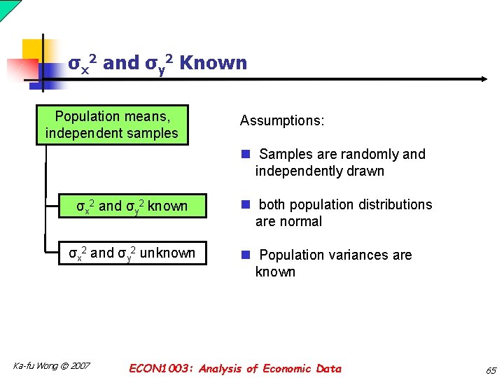
σx 2 and σy 2 Known Population means, independent samples Assumptions: n Samples are randomly and independently drawn σx 2 and σy 2 known σx 2 and σy 2 unknown Ka-fu Wong © 2007 n both population distributions are normal n Population variances are known ECON 1003: Analysis of Economic Data 65

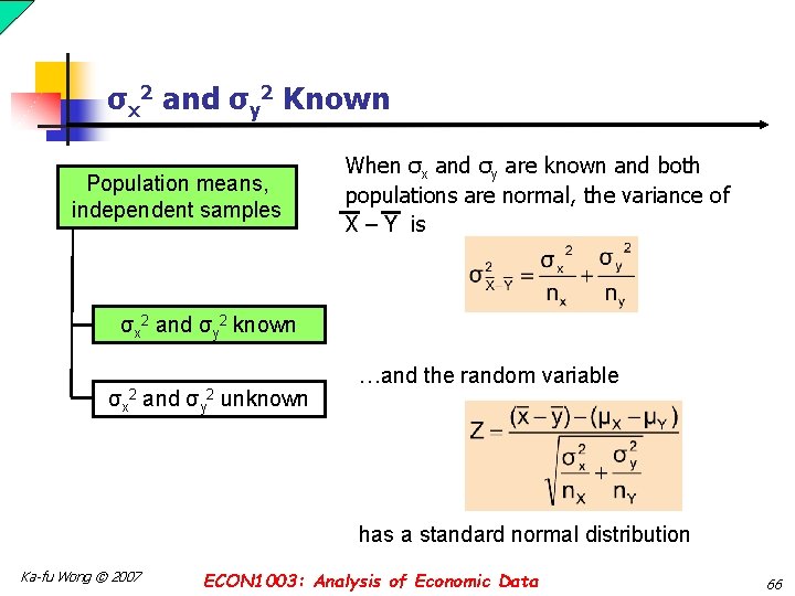
σx 2 and σy 2 Known Population means, independent samples When σx and σy are known and both populations are normal, the variance of X – Y is σx 2 and σy 2 known σx 2 and σy 2 unknown …and the random variable has a standard normal distribution Ka-fu Wong © 2007 ECON 1003: Analysis of Economic Data 66

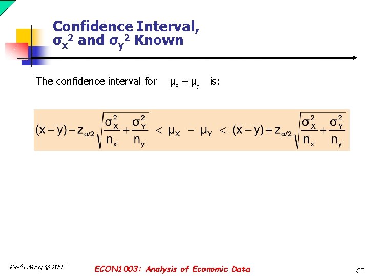
Confidence Interval, σx 2 and σy 2 Known The confidence interval for Ka-fu Wong © 2007 μx – μy is: ECON 1003: Analysis of Economic Data 67

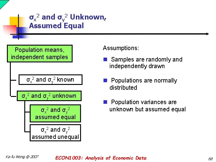
σx 2 and σy 2 Unknown, Assumed Equal Population means, independent samples σx 2 and σy 2 known σx 2 and σy 2 unknown σx 2 and σy 2 assumed equal Assumptions: n Samples are randomly and independently drawn n Populations are normally distributed n Population variances are unknown but assumed equal σx 2 and σy 2 assumed unequal Ka-fu Wong © 2007 ECON 1003: Analysis of Economic Data 68

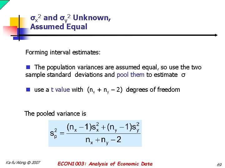
σx 2 and σy 2 Unknown, Assumed Equal Forming interval estimates: n The population variances are assumed equal, so use the two sample standard deviations and pool them to estimate σ n use a t value with (nx + ny – 2) degrees of freedom The pooled variance is Ka-fu Wong © 2007 ECON 1003: Analysis of Economic Data 69

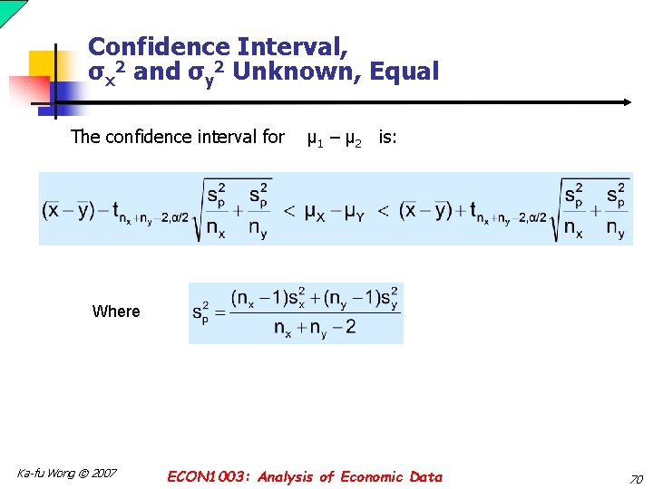
Confidence Interval, σx 2 and σy 2 Unknown, Equal The confidence interval for μ 1 – μ 2 is: Where Ka-fu Wong © 2007 ECON 1003: Analysis of Economic Data 70

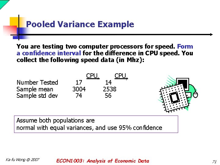
Pooled Variance Example You are testing two computer processors for speed. Form a confidence interval for the difference in CPU speed. You collect the following speed data (in Mhz): Number Tested Sample mean Sample std dev 17 3004 74 CPUx CPUy 14 2538 56 Assume both populations are normal with equal variances, and use 95% confidence Ka-fu Wong © 2007 ECON 1003: Analysis of Economic Data 71

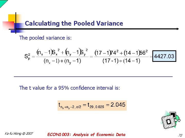
Calculating the Pooled Variance The pooled variance is: The t value for a 95% confidence interval is: Ka-fu Wong © 2007 ECON 1003: Analysis of Economic Data 72

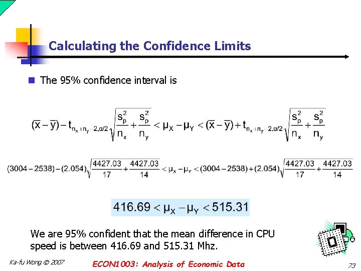
Calculating the Confidence Limits n The 95% confidence interval is We are 95% confident that the mean difference in CPU speed is between 416. 69 and 515. 31 Mhz. Ka-fu Wong © 2007 ECON 1003: Analysis of Economic Data 73

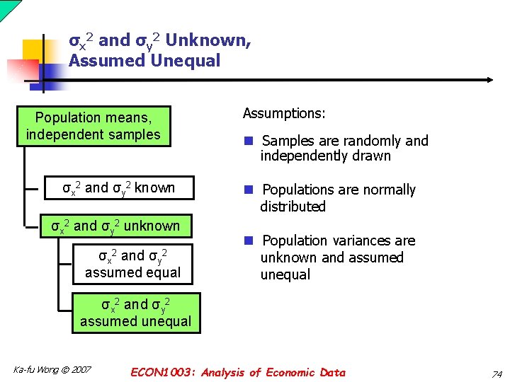
σx 2 and σy 2 Unknown, Assumed Unequal Population means, independent samples σx 2 and σy 2 known σx 2 and σy 2 unknown σx 2 and σy 2 assumed equal Assumptions: n Samples are randomly and independently drawn n Populations are normally distributed n Population variances are unknown and assumed unequal σx 2 and σy 2 assumed unequal Ka-fu Wong © 2007 ECON 1003: Analysis of Economic Data 74

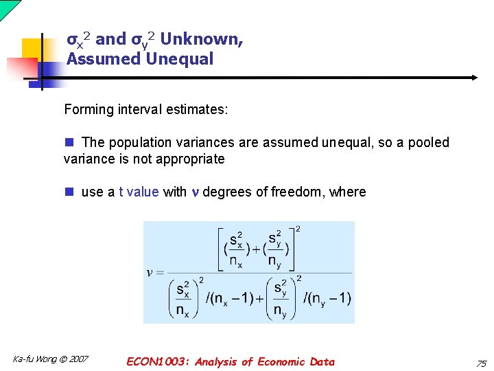
σx 2 and σy 2 Unknown, Assumed Unequal Forming interval estimates: n The population variances are assumed unequal, so a pooled variance is not appropriate n use a t value with degrees of freedom, where Ka-fu Wong © 2007 ECON 1003: Analysis of Economic Data 75

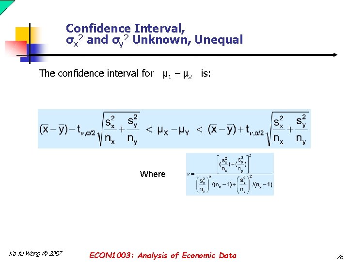
Confidence Interval, σx 2 and σy 2 Unknown, Unequal The confidence interval for μ 1 – μ 2 is: Where Ka-fu Wong © 2007 ECON 1003: Analysis of Economic Data 76

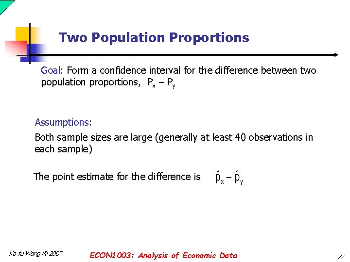
Two Population Proportions Goal: Form a confidence interval for the difference between two population proportions, Px – Py Assumptions: Both sample sizes are large (generally at least 40 observations in each sample) The point estimate for the difference is Ka-fu Wong © 2007 ECON 1003: Analysis of Economic Data 77

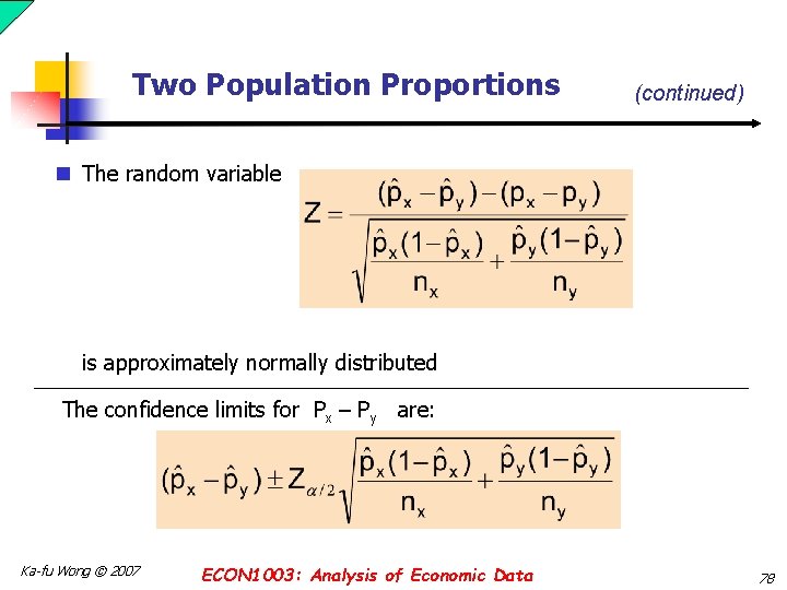
Two Population Proportions (continued) n The random variable is approximately normally distributed The confidence limits for Px – Py are: Ka-fu Wong © 2007 ECON 1003: Analysis of Economic Data 78

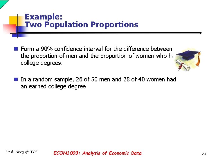
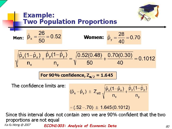
Example: Two Population Proportions n Form a 90% confidence interval for the difference between the proportion of men and the proportion of women who have college degrees. n In a random sample, 26 of 50 men and 28 of 40 women had an earned college degree Ka-fu Wong © 2007 ECON 1003: Analysis of Economic Data 79

Example: Two Population Proportions Women: Men: For 90% confidence, Z /2 = 1. 645 The confidence limits are: Since this interval does not contain zero we are 90% confident that the two proportions are not equal Ka-fu Wong © 2007 ECON 1003: Analysis of Economic Data 80

Confidence Intervals for the Population Variance n The confidence interval is based on the sample variance, s 2 n Assumed: the population is normally distributed The random variable follows a chi-square distribution with (n – 1) degrees of freedom The chi-square value denotes the number for which Ka-fu Wong © 2007 ECON 1003: Analysis of Economic Data 81

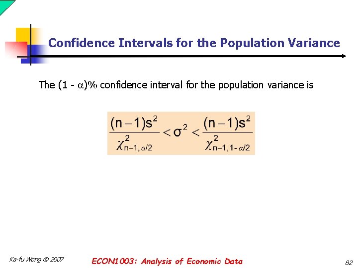
Confidence Intervals for the Population Variance The (1 - )% confidence interval for the population variance is Ka-fu Wong © 2007 ECON 1003: Analysis of Economic Data 82

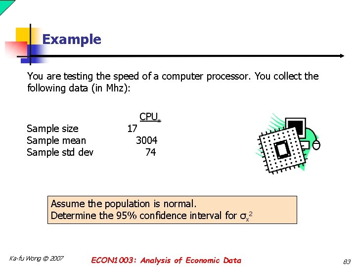
Example You are testing the speed of a computer processor. You collect the following data (in Mhz): Sample size Sample mean Sample std dev CPUx 17 3004 74 Assume the population is normal. Determine the 95% confidence interval for σx 2 Ka-fu Wong © 2007 ECON 1003: Analysis of Economic Data 83

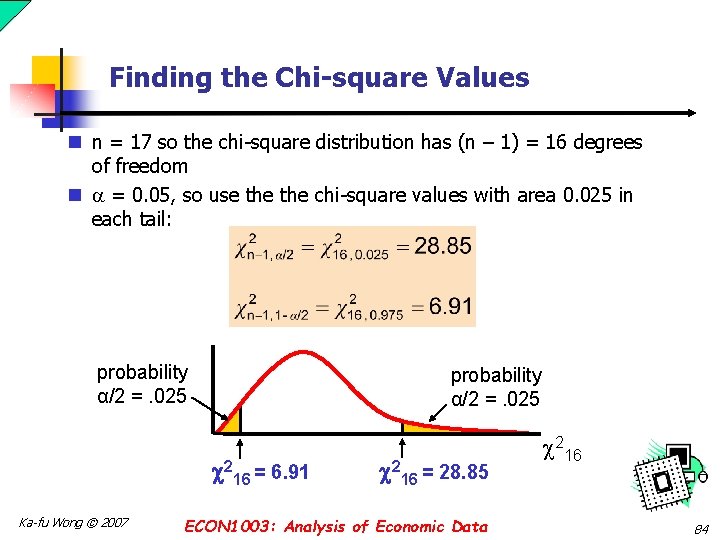
Finding the Chi-square Values n n = 17 so the chi-square distribution has (n – 1) = 16 degrees of freedom n = 0. 05, so use the chi-square values with area 0. 025 in each tail: probability α/2 =. 025 216 = 6. 91 Ka-fu Wong © 2007 216 = 28. 85 ECON 1003: Analysis of Economic Data 216 84

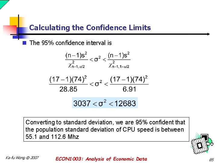
Calculating the Confidence Limits n The 95% confidence interval is Converting to standard deviation, we are 95% confident that the population standard deviation of CPU speed is between 55. 1 and 112. 6 Mhz Ka-fu Wong © 2007 ECON 1003: Analysis of Economic Data 85

Lesson 9: Confidence Intervals and Tests of Hypothesis Two or more samples - END - Ka-fu Wong © 2007 ECON 1003: Analysis of Economic Data Lesson 9 -86