Lesson 8 Gauss Jordan Elimination Serial and Parallel

Lesson 8 Gauss Jordan Elimination Serial and Parallel algorithms

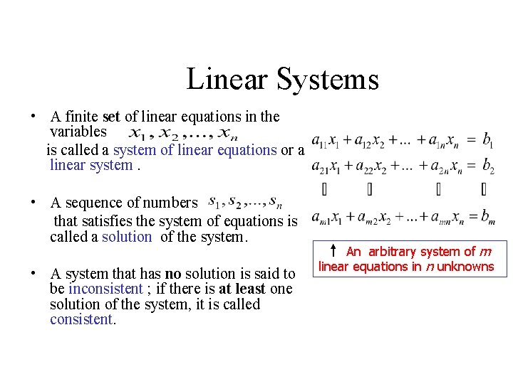
Linear Systems • A finite set of linear equations in the variables is called a system of linear equations or a linear system. • A sequence of numbers that satisfies the system of equations is called a solution of the system. • A system that has no solution is said to be inconsistent ; if there is at least one solution of the system, it is called consistent. An arbitrary system of m linear equations in n unknowns

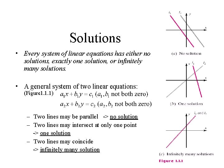
Solutions • Every system of linear equations has either no solutions, exactly one solution, or infinitely many solutions. • A general system of two linear equations: (Figure 1. 1. 1) – Two lines may be parallel -> no solution – Two lines may intersect at only one point -> one solution – Two lines may coincide -> infinitely many solution

Systems of Linear Equations • Systems of linear algebraic equations may represent too much, or too little or just the right amount of information to determine values of the variables constituting solutions. • Using Gauss-Jordan elimination we can determine whether the system has many solutions, a unique solution or none at all.

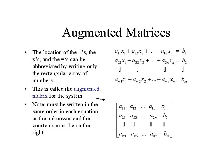
Augmented Matrices • The location of the +’s, the x’s, and the =‘s can be abbreviated by writing only the rectangular array of numbers. • This is called the augmented matrix for the system. • Note: must be written in the same order in each equation as the unknowns and the constants must be on the right.

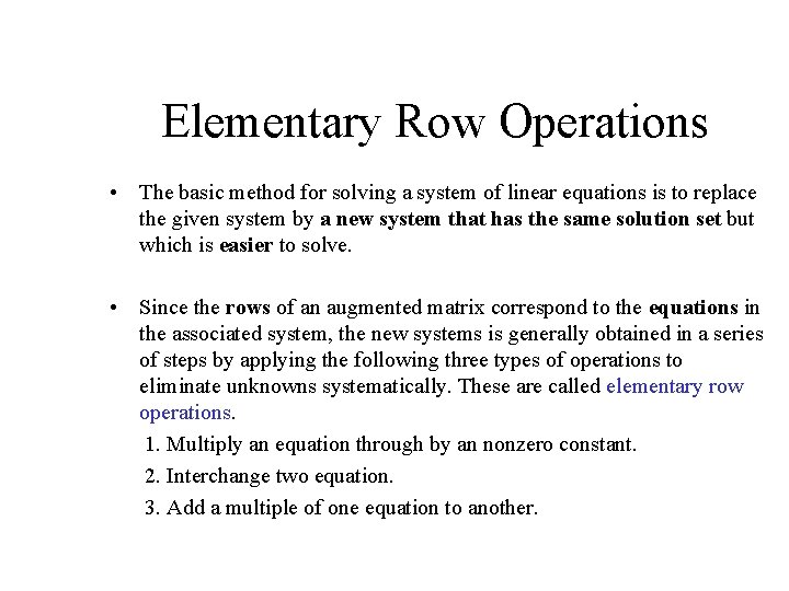
Elementary Row Operations • The basic method for solving a system of linear equations is to replace the given system by a new system that has the same solution set but which is easier to solve. • Since the rows of an augmented matrix correspond to the equations in the associated system, the new systems is generally obtained in a series of steps by applying the following three types of operations to eliminate unknowns systematically. These are called elementary row operations. 1. Multiply an equation through by an nonzero constant. 2. Interchange two equation. 3. Add a multiple of one equation to another.

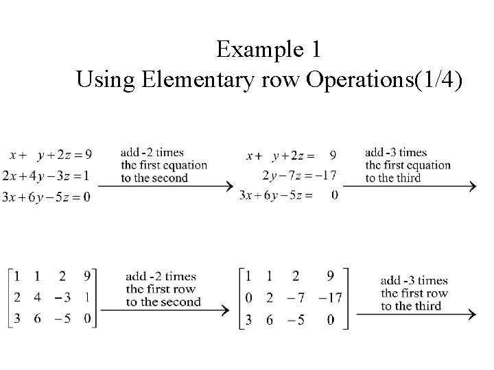
Example 1 Using Elementary row Operations(1/4)

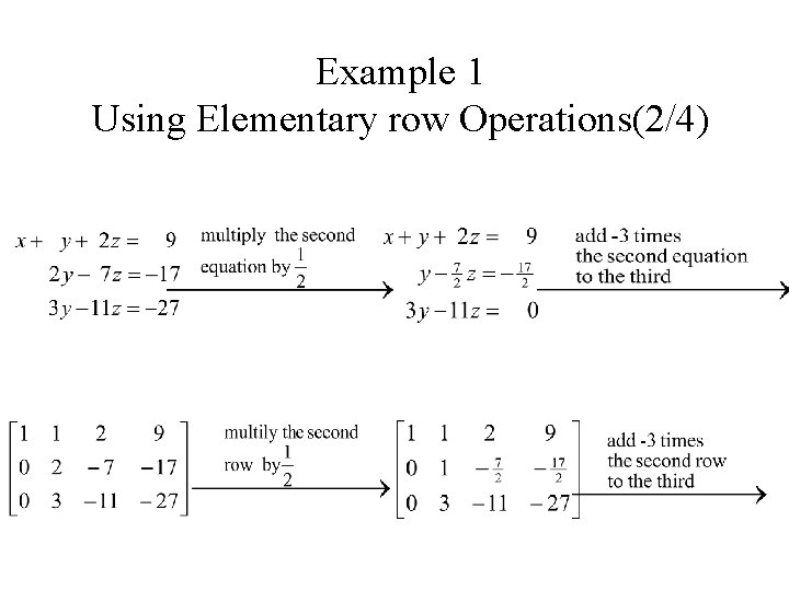
Example 1 Using Elementary row Operations(2/4)

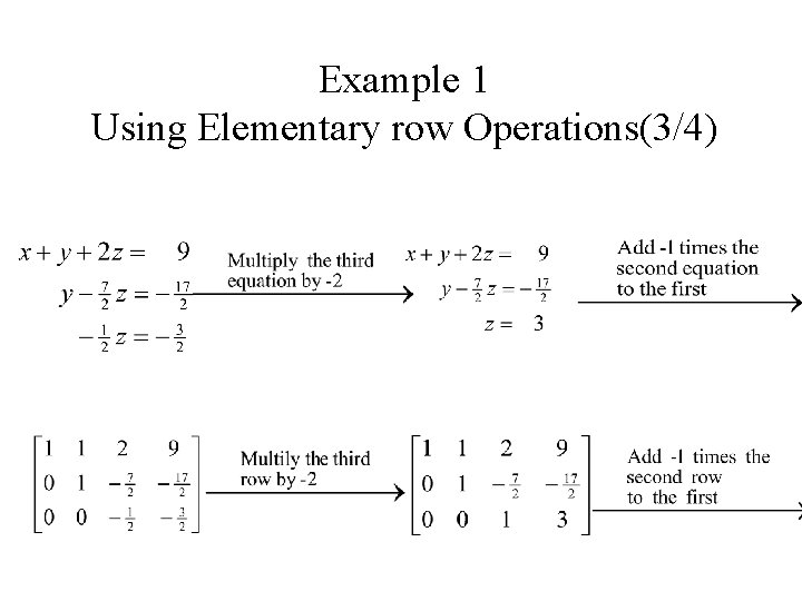
Example 1 Using Elementary row Operations(3/4)

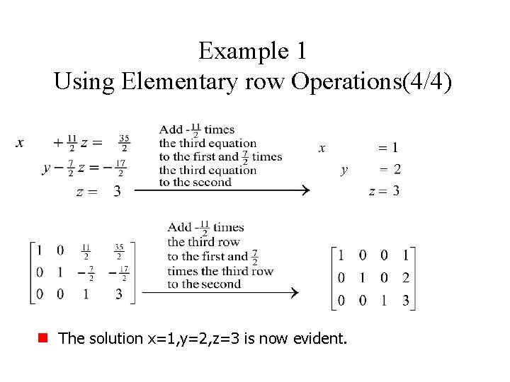
Example 1 Using Elementary row Operations(4/4) n The solution x=1, y=2, z=3 is now evident.

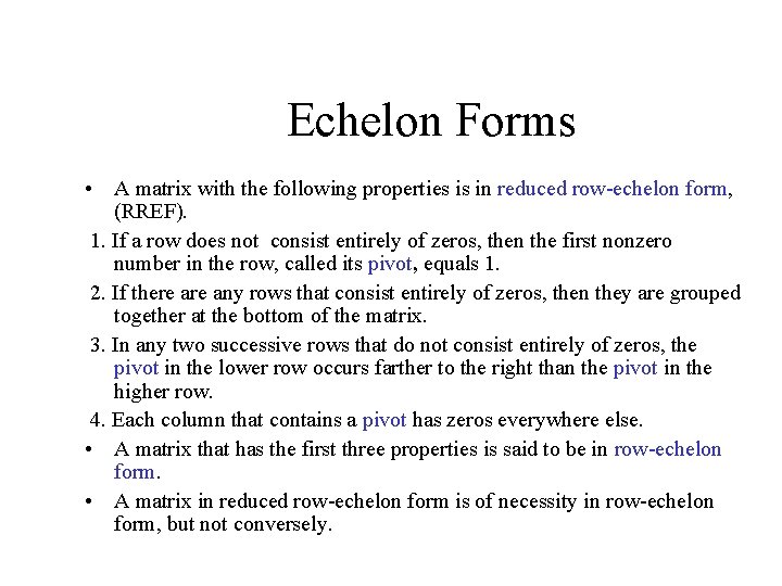
Echelon Forms • A matrix with the following properties is in reduced row-echelon form, (RREF). 1. If a row does not consist entirely of zeros, then the first nonzero number in the row, called its pivot, equals 1. 2. If there any rows that consist entirely of zeros, then they are grouped together at the bottom of the matrix. 3. In any two successive rows that do not consist entirely of zeros, the pivot in the lower row occurs farther to the right than the pivot in the higher row. 4. Each column that contains a pivot has zeros everywhere else. • A matrix that has the first three properties is said to be in row-echelon form. • A matrix in reduced row-echelon form is of necessity in row-echelon form, but not conversely.

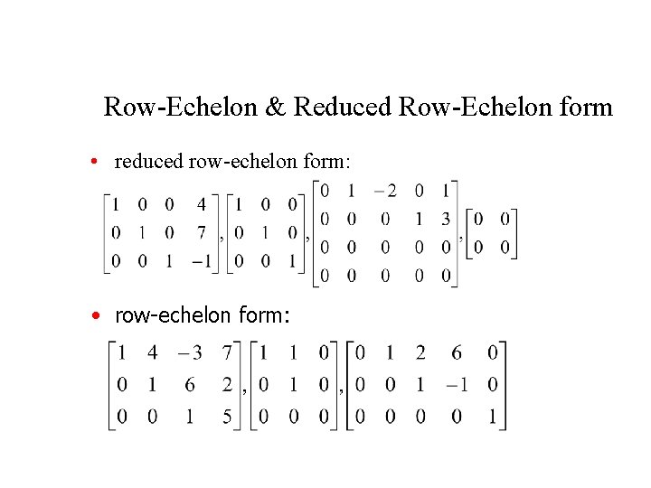
Row-Echelon & Reduced Row-Echelon form • reduced row-echelon form: • row-echelon form:

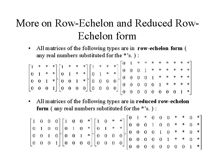
More on Row-Echelon and Reduced Row. Echelon form • All matrices of the following types are in row-echelon form ( any real numbers substituted for the *’s. ) : • All matrices of the following types are in reduced row-echelon form ( any real numbers substituted for the *’s. ) :

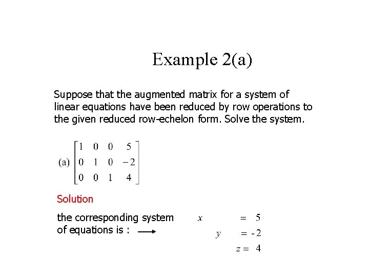
Example 2(a) Suppose that the augmented matrix for a system of linear equations have been reduced by row operations to the given reduced row-echelon form. Solve the system. Solution the corresponding system of equations is :

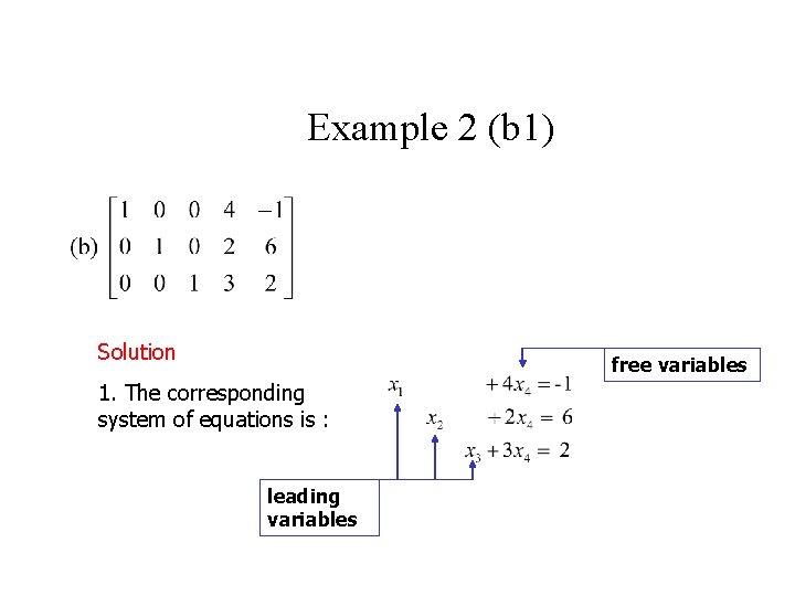
Example 2 (b 1) Solution free variables 1. The corresponding system of equations is : leading variables

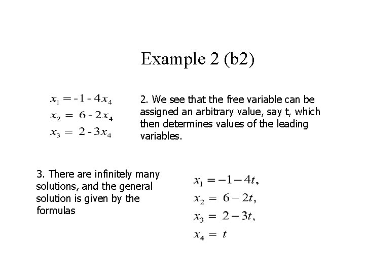
Example 2 (b 2) 2. We see that the free variable can be assigned an arbitrary value, say t, which then determines values of the leading variables. 3. There are infinitely many solutions, and the general solution is given by the formulas

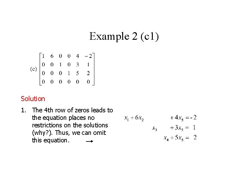
Example 2 (c 1) Solution 1. The 4 th row of zeros leads to the equation places no restrictions on the solutions (why? ). Thus, we can omit this equation.

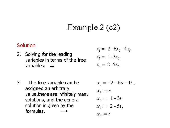
Example 2 (c 2) Solution 2. Solving for the leading variables in terms of the free variables: 3. The free variable can be assigned an arbitrary value, there are infinitely many solutions, and the general solution is given by the formulas.

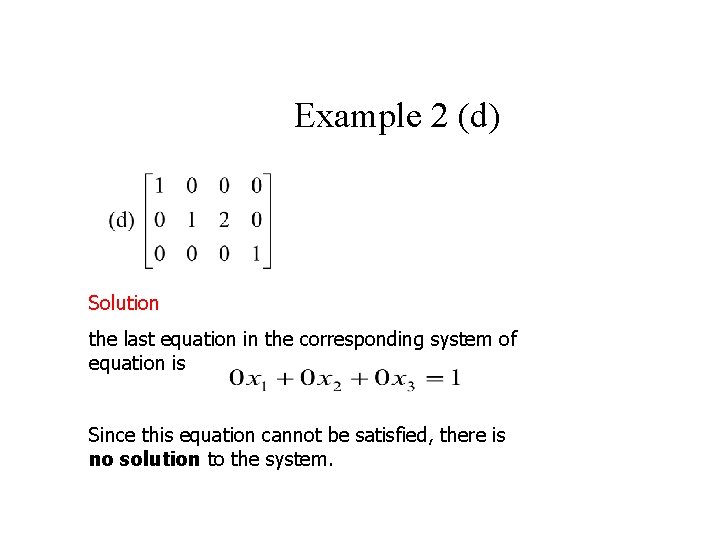
Example 2 (d) Solution the last equation in the corresponding system of equation is Since this equation cannot be satisfied, there is no solution to the system.

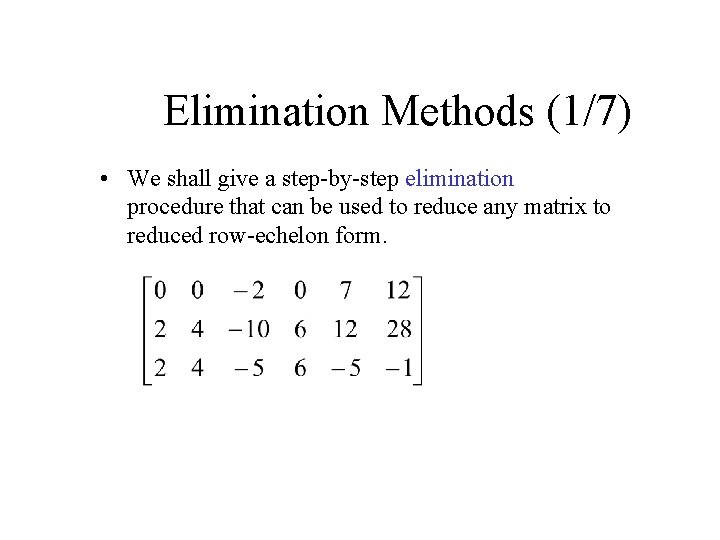
Elimination Methods (1/7) • We shall give a step-by-step elimination procedure that can be used to reduce any matrix to reduced row-echelon form.

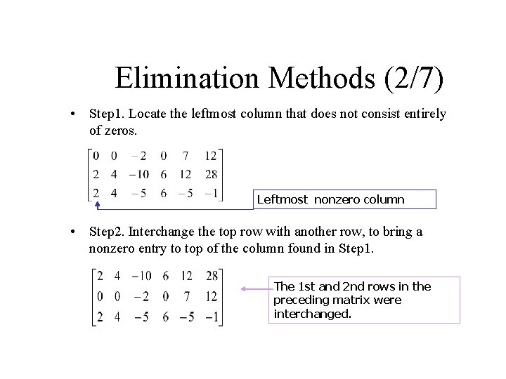
Elimination Methods (2/7) • Step 1. Locate the leftmost column that does not consist entirely of zeros. Leftmost nonzero column • Step 2. Interchange the top row with another row, to bring a nonzero entry to top of the column found in Step 1. The 1 st and 2 nd rows in the preceding matrix were interchanged.

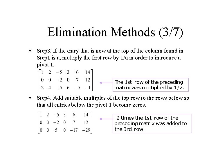
Elimination Methods (3/7) • Step 3. If the entry that is now at the top of the column found in Step 1 is a, multiply the first row by 1/a in order to introduce a pivot 1. The 1 st row of the preceding matrix was multiplied by 1/2. • Step 4. Add suitable multiples of the top row to the rows below so that all entries below the pivot 1 become zeros. -2 times the 1 st row of the preceding matrix was added to the 3 rd row.

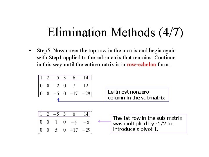
Elimination Methods (4/7) • Step 5. Now cover the top row in the matrix and begin again with Step 1 applied to the sub-matrix that remains. Continue in this way until the entire matrix is in row-echelon form. Leftmost nonzero column in the submatrix The 1 st row in the sub-matrix was multiplied by -1/2 to introduce a pivot 1.

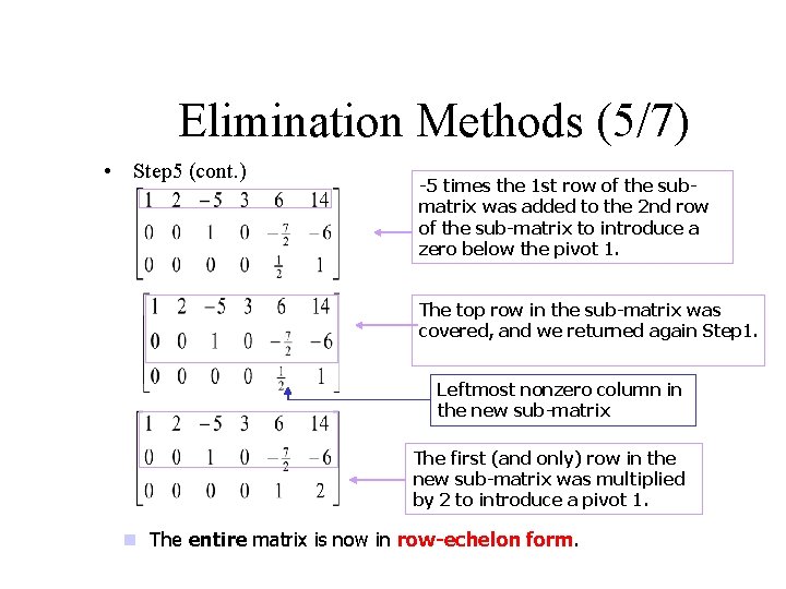
Elimination Methods (5/7) • Step 5 (cont. ) -5 times the 1 st row of the submatrix was added to the 2 nd row of the sub-matrix to introduce a zero below the pivot 1. The top row in the sub-matrix was covered, and we returned again Step 1. Leftmost nonzero column in the new sub-matrix The first (and only) row in the new sub-matrix was multiplied by 2 to introduce a pivot 1. n The entire matrix is now in row-echelon form.

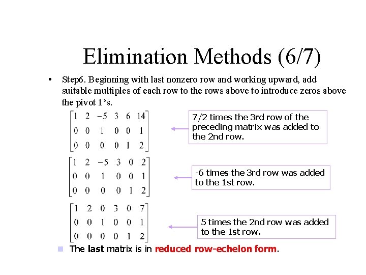
Elimination Methods (6/7) • Step 6. Beginning with last nonzero row and working upward, add suitable multiples of each row to the rows above to introduce zeros above the pivot 1’s. 7/2 times the 3 rd row of the preceding matrix was added to the 2 nd row. -6 times the 3 rd row was added to the 1 st row. 5 times the 2 nd row was added to the 1 st row. n The last matrix is in reduced row-echelon form.

Elimination Methods (7/7) • Step 1~Step 5: the above procedure produces a rowechelon form and is called Gaussian elimination. • Step 1~Step 6: the above procedure produces a reduced row-echelon form and is called Gaussian-Jordan elimination. • Every matrix has a unique reduced row-echelon form but a row-echelon form of a given matrix is not unique.

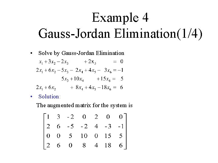
Example 4 Gauss-Jordan Elimination(1/4) • Solve by Gauss-Jordan Elimination • Solution: The augmented matrix for the system is

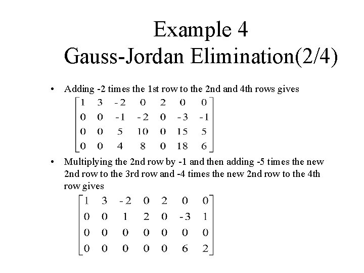
Example 4 Gauss-Jordan Elimination(2/4) • Adding -2 times the 1 st row to the 2 nd and 4 th rows gives • Multiplying the 2 nd row by -1 and then adding -5 times the new 2 nd row to the 3 rd row and -4 times the new 2 nd row to the 4 th row gives

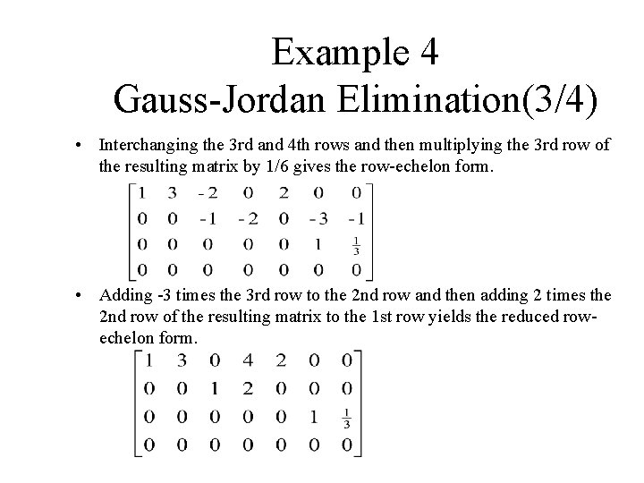
Example 4 Gauss-Jordan Elimination(3/4) • Interchanging the 3 rd and 4 th rows and then multiplying the 3 rd row of the resulting matrix by 1/6 gives the row-echelon form. • Adding -3 times the 3 rd row to the 2 nd row and then adding 2 times the 2 nd row of the resulting matrix to the 1 st row yields the reduced rowechelon form.

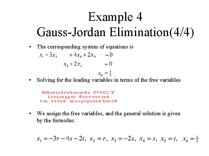
Example 4 Gauss-Jordan Elimination(4/4) • The corresponding system of equations is • Solving for the leading variables in terms of the free variables • We assign the free variables, and the general solution is given by the formulas:

Back-Substitution • It is sometimes preferable to solve a system of linear equations by using Gaussian elimination to bring the augmented matrix into row-echelon form without continuing all the way to the reduced row-echelon form. • When this is done, the corresponding system of equations can be solved by by a technique called back-substitution. • Example 5

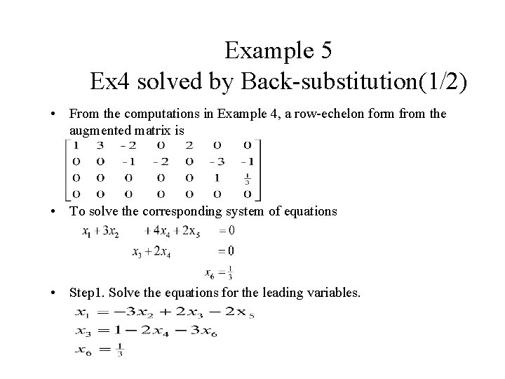
Example 5 Ex 4 solved by Back-substitution(1/2) • From the computations in Example 4, a row-echelon form from the augmented matrix is • To solve the corresponding system of equations • Step 1. Solve the equations for the leading variables.

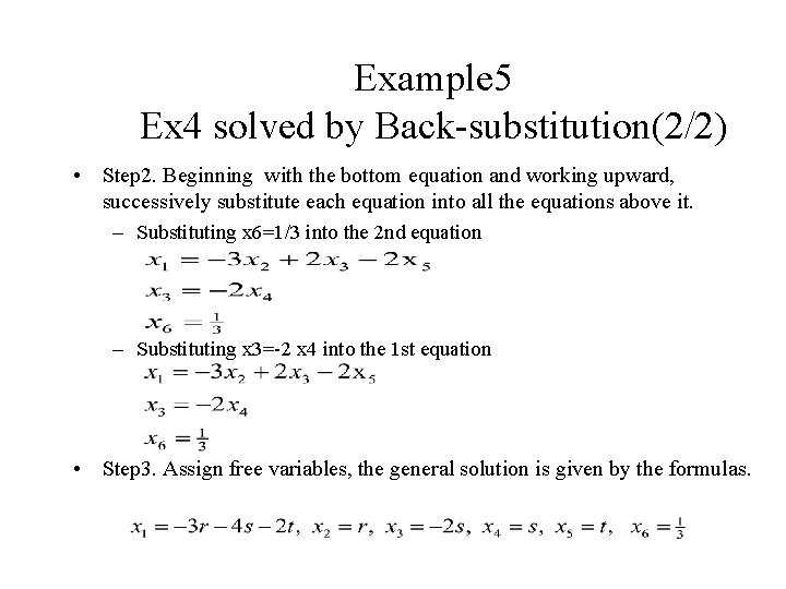
Example 5 Ex 4 solved by Back-substitution(2/2) • Step 2. Beginning with the bottom equation and working upward, successively substitute each equation into all the equations above it. – Substituting x 6=1/3 into the 2 nd equation – Substituting x 3=-2 x 4 into the 1 st equation • Step 3. Assign free variables, the general solution is given by the formulas.

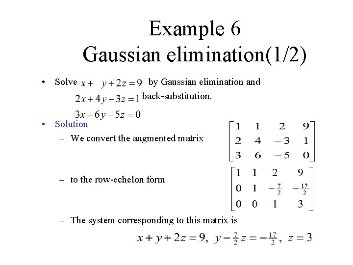
Example 6 Gaussian elimination(1/2) • Solve by Gaussian elimination and back-substitution. • Solution – We convert the augmented matrix – to the row-echelon form – The system corresponding to this matrix is

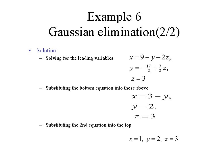
Example 6 Gaussian elimination(2/2) • Solution – Solving for the leading variables – Substituting the bottom equation into those above – Substituting the 2 nd equation into the top