Lesson 8 Basic Monte Carlo integration We begin

Lesson 8: Basic Monte Carlo integration We begin the 2 nd phase of our course: Study of general mathematics of MC Consists of a progression: • • • Monte Carlo evaluation of integrals (4 ways) Basic numerical analysis framework (to explain the 4 ways) MC evaluation of integral equations Generalization of this technique to solve general differential equation sets 1

Monte Carlo Integration Next set of mathematical tools: MC integration Our study so far of sampling from distributions has provided us with the tools for MC simulation MC integration will provide: • • More rigorous ideas of keeping score Basic mathematical underpinnings of variance reduction. “Abstract” approach to MC problem: ALMOST ALL MC PROBLEMS ARE INTEGRATIONS Development of four particular methods using the framework. 2

Four particular integration methods • We will now go over four particular variations on this theme: 1. Rejection method 2. Averaging method 3. Control variates method 4. Importance sampling method 3

Rejection method • • • This is a similar approach to the use of rejection methods in picking from a distribution. It is a "dart board" method in which we estimate the area under a functional curve by containing the curve in a rectangular "box", picking a point randomly in the box, and scoring 0 if it misses (i. e. , is above the curve) or the full rectangular area if it hits (i. e. , is below the curve). As before, we have to specify an upper bound of the function, , and then proceed by: 4

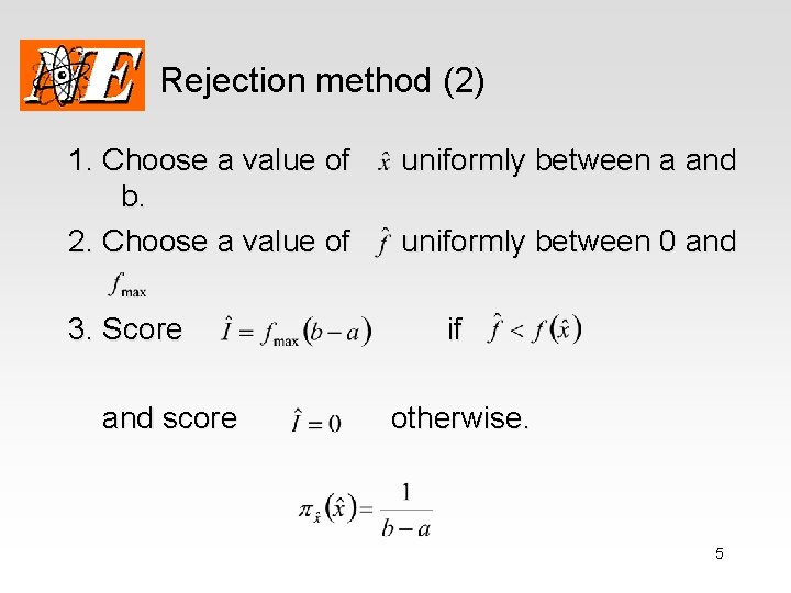
Rejection method (2) 1. Choose a value of b. 2. Choose a value of 3. Score and score uniformly between a and uniformly between 0 and if otherwise. 5

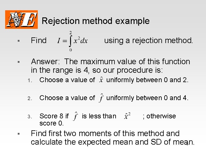
Rejection method example § Find § Answer: The maximum value of this function in the range is 4, so our procedure is: § using a rejection method. 1. Choose a value of uniformly between 0 and 2. Choose a value of uniformly between 0 and 4. 3. Score 8 if score 0. is less than ; otherwise Find first two moments of this method and calculate the expected mean and SD of mean. 6

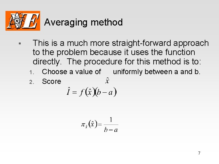
Averaging method § This is a much more straight-forward approach to the problem because it uses the function directly. The procedure for this method is to: 1. 2. Choose a value of Score uniformly between a and b. 7

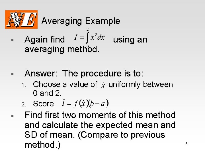
Averaging Example § Again find averaging method. § Answer: The procedure is to: 1. 2. § Choose a value of 0 and 2. Score using an uniformly between Find first two moments of this method and calculate the expected mean and SD of mean. (Compare to previous method. ) 8

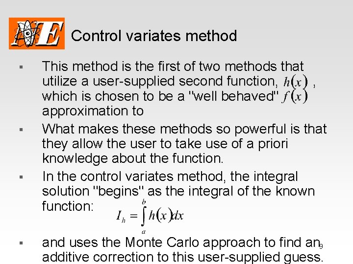
Control variates method § § This method is the first of two methods that utilize a user-supplied second function, , which is chosen to be a "well behaved" approximation to What makes these methods so powerful is that they allow the user to take use of a priori knowledge about the function. In the control variates method, the integral solution "begins" as the integral of the known function: and uses the Monte Carlo approach to find an 9 additive correction to this user-supplied guess.

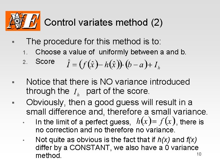
Control variates method (2) The procedure for this method is to: § 1. 2. Choose a value of uniformly between a and b. Score Notice that there is NO variance introduced through the part of the score. Obviously, then a good guess will result in a small difference and, therefore a small variance. § § • • In the limit of a perfect guess, , there is no correction and no therefore no variance. Not quite as obvious is the fact that if h(x) and f(x) differ by a CONSTANT, we also have a 0 variance 10 method.

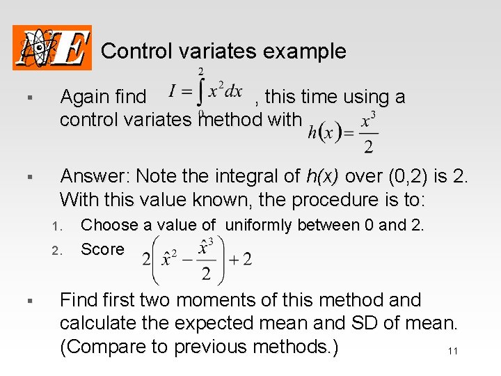
Control variates example § Again find , this time using a control variates method with § Answer: Note the integral of h(x) over (0, 2) is 2. With this value known, the procedure is to: 1. 2. § Choose a value of uniformly between 0 and 2. Score Find first two moments of this method and calculate the expected mean and SD of mean. (Compare to previous methods. ) 11

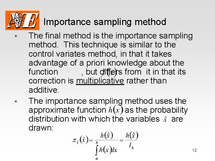
Importance sampling method § § The final method is the importance sampling method. This technique is similar to the control variates method, in that it takes advantage of a priori knowledge about the function , but differs from it in that its correction is multiplicative rather than additive. The importance sampling method uses the approximate function as the probability distribution with which the variables are drawn: 12

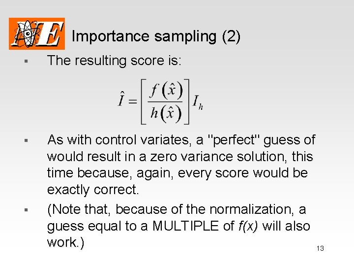
Importance sampling (2) § The resulting score is: § As with control variates, a "perfect" guess of would result in a zero variance solution, this time because, again, every score would be exactly correct. (Note that, because of the normalization, a guess equal to a MULTIPLE of f(x) will also work. ) 13 §

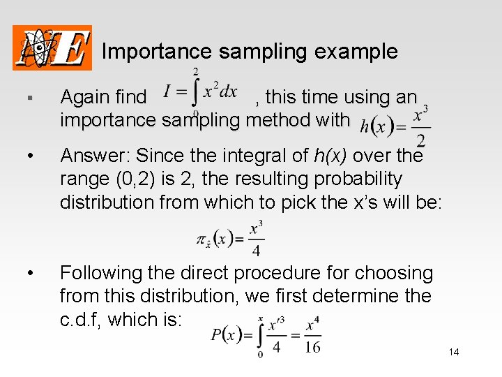
Importance sampling example § Again find , this time using an importance sampling method with • Answer: Since the integral of h(x) over the range (0, 2) is 2, the resulting probability distribution from which to pick the x’s will be: • Following the direct procedure for choosing from this distribution, we first determine the c. d. f, which is: 14

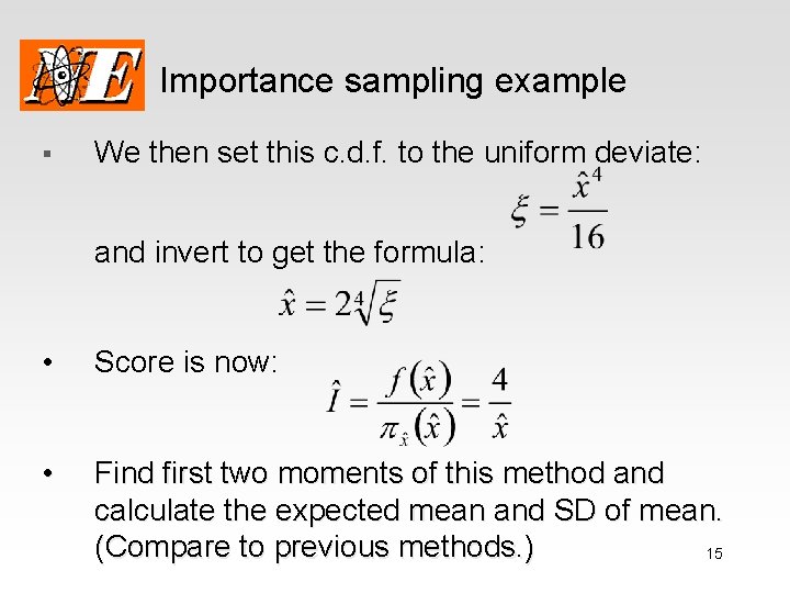
Importance sampling example § We then set this c. d. f. to the uniform deviate: and invert to get the formula: • Score is now: • Find first two moments of this method and calculate the expected mean and SD of mean. (Compare to previous methods. ) 15

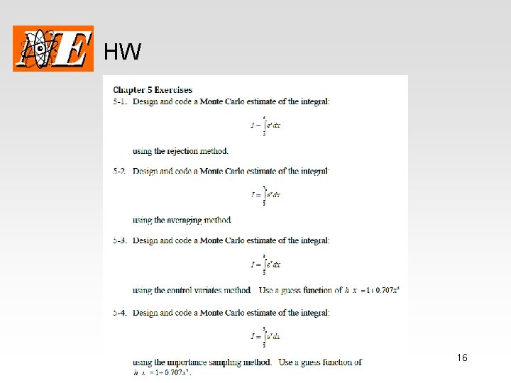
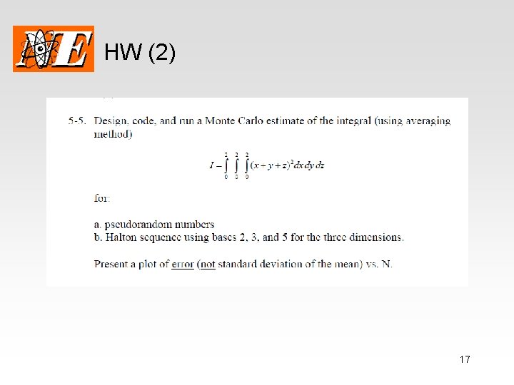
HW 16

HW (2) 17

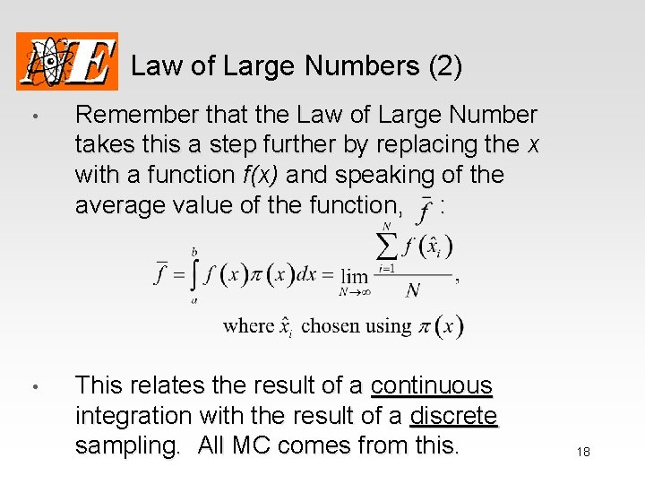
Law of Large Numbers (2) • Remember that the Law of Large Number takes this a step further by replacing the x with a function f(x) and speaking of the average value of the function, : • This relates the result of a continuous integration with the result of a discrete sampling. All MC comes from this. 18

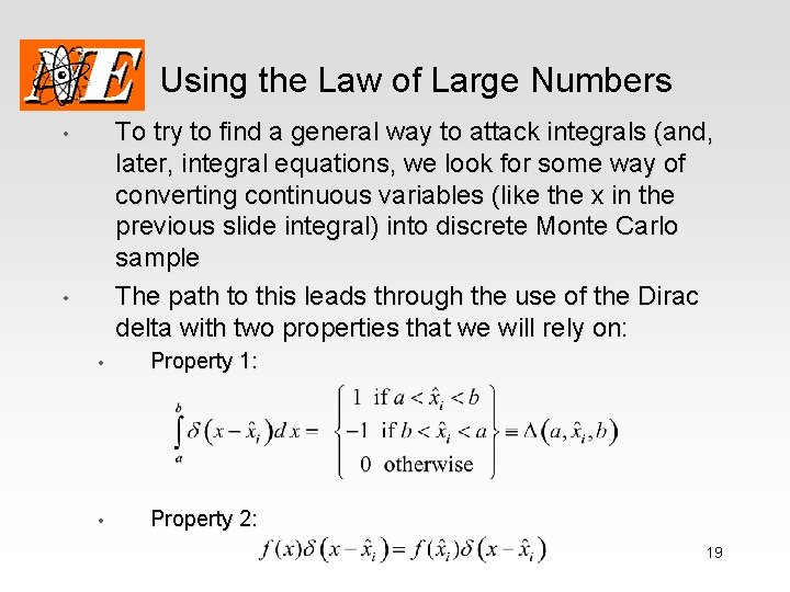
Using the Law of Large Numbers To try to find a general way to attack integrals (and, later, integral equations, we look for some way of converting continuous variables (like the x in the previous slide integral) into discrete Monte Carlo sample The path to this leads through the use of the Dirac delta with two properties that we will rely on: • • • Property 1: • Property 2: 19

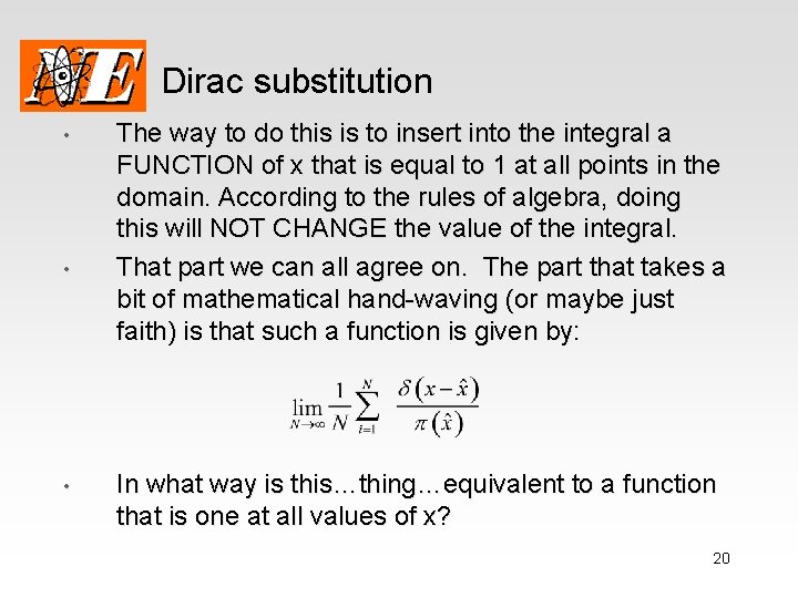
Dirac substitution • • • The way to do this is to insert into the integral a FUNCTION of x that is equal to 1 at all points in the domain. According to the rules of algebra, doing this will NOT CHANGE the value of the integral. That part we can all agree on. The part that takes a bit of mathematical hand-waving (or maybe just faith) is that such a function is given by: In what way is this…thing…equivalent to a function that is one at all values of x? 20

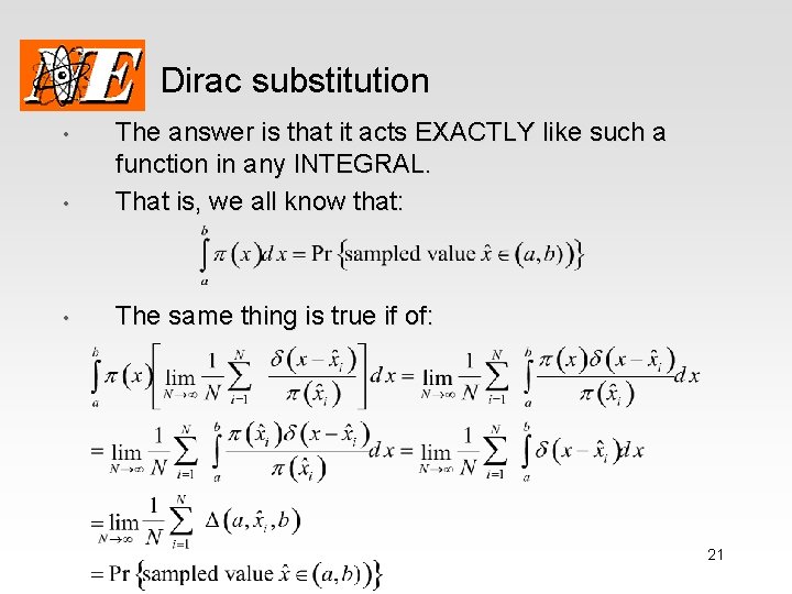
Dirac substitution • The answer is that it acts EXACTLY like such a function in any INTEGRAL. That is, we all know that: • The same thing is true if of: • 21

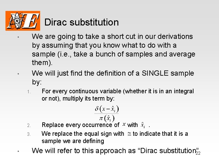
Dirac substitution We are going to take a short cut in our derivations by assuming that you know what to do with a sample (i. e. , take a bunch of samples and average them). We will just find the definition of a SINGLE sample by: • • 1. For every continuous variable (whether it is in an integral or not), multiply its term by: 2. Replace every occurrence of with. We replace the equal sign with to indicate that it is a sample we are defining 3. • We will refer to this approach as “Dirac substitution” 22

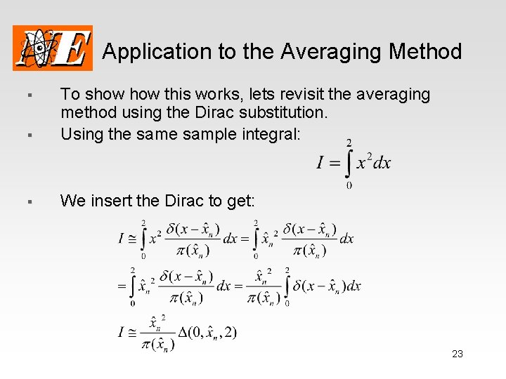
Application to the Averaging Method § To show this works, lets revisit the averaging method using the Dirac substitution. Using the sample integral: § We insert the Dirac to get: § 23

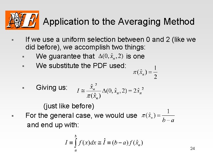
Application to the Averaging Method § If we use a uniform selection between 0 and 2 (like we did before), we accomplish two things: § We guarantee that is one § We substitute the PDF used: § § Giving us: (just like before) For the general case, we would use and end up with: 24

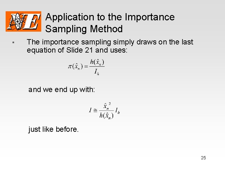
Application to the Importance Sampling Method § The importance sampling simply draws on the last equation of Slide 21 and uses: and we end up with: just like before. 25