Lesson 74 Introduction to Taylor Maclaurin Series HL

RECAP From last lesson: (1) We CAN model a function using a power series

Suppose we wanted to find a fourth degree polynomial of the form: that approximates

We are going to start by making two assumptions: (a) Let’s assume that

If we plot both functions, we see that near zero the functions match very

Our polynomial: has the form: or: This pattern occurs no matter what the original

Maclaurin Series: (generated by f at ) If we want to center the series

The more terms we add, the better our approximation. Hint: On the TI-89, the

example: Rather than start from scratch, we can use the function that we already

There are some Maclaurin series that occur often enough that they should be memorized.

When referring to Taylor polynomials, we can talk about number of terms, order or

Slides: 19

Download presentation

Lesson 74 – Introduction to Taylor & Maclaurin Series HL Math - Santowski

RECAP From last lesson: (1) We CAN model a function using a power series (2) These power series are based upon geometric series (3) Therefore, the functions that we can “work with” at this stage are variations of the function: Question Can we develop a more “general” approach to developing a series in order to represent ANY function?

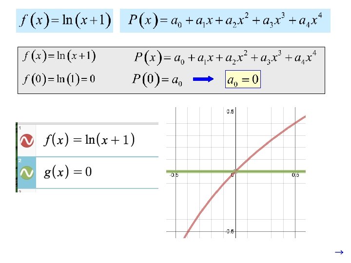
Suppose we wanted to find a fourth degree polynomial of the form: that approximates the behavior of BUT HOW do we do that? ? ? at

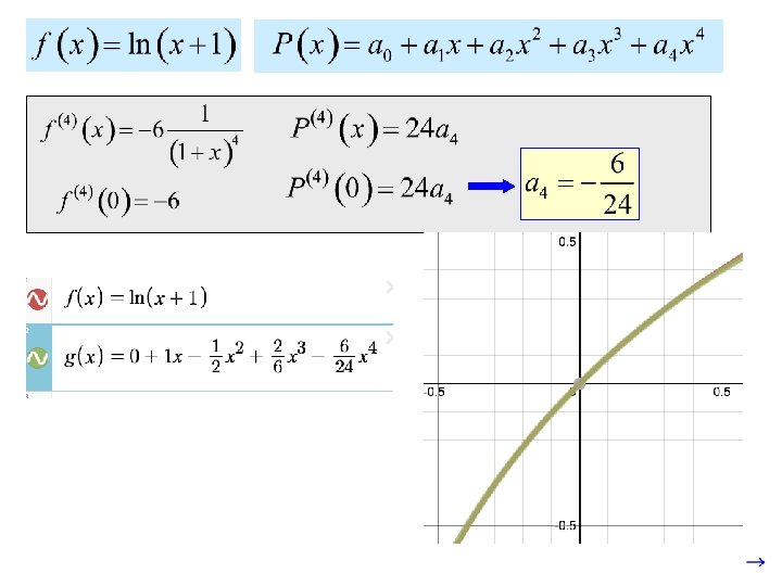
We are going to start by making two assumptions: (a) Let’s assume that the function y = f(x) does in fact have a power series representation about x = a (in this case, f(x) = ln(x + 1) at x = 0 ) (b) Next we will assume that the function y = f(x) has derivatives of every order and that we can in fact find them all

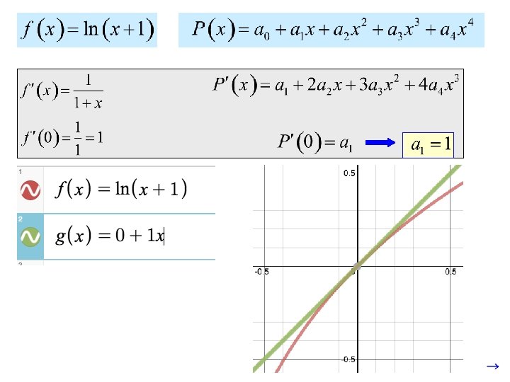
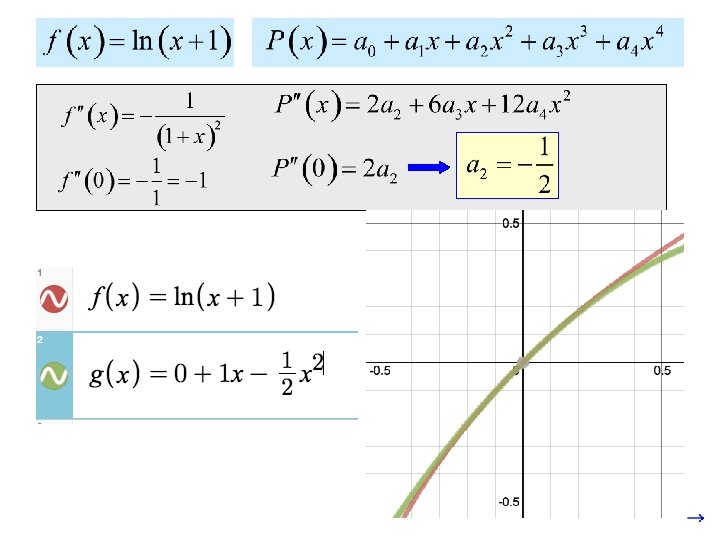
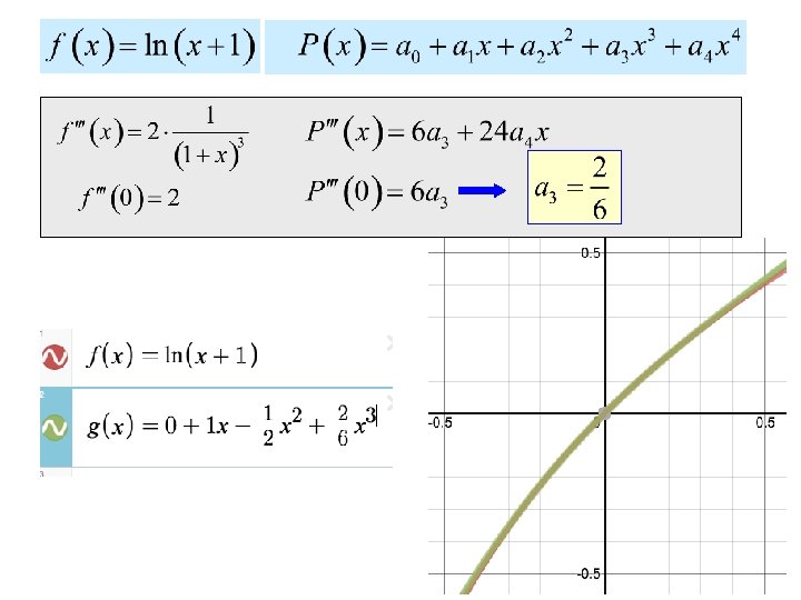
Suppose we wanted to find a fourth degree polynomial of the form: that approximates the behavior of If we make at , and the first, second, third and fourth derivatives the same, then we would have a pretty good approximation.

If we plot both functions, we see that near zero the functions match very well!

Our polynomial: has the form: or: This pattern occurs no matter what the original function was!

Maclaurin Series: (generated by f at ) If we want to center the series (and it’s graph) at some point other than zero, we get the Taylor Series: (generated by f at )

example:

The more terms we add, the better our approximation. Hint: On the TI-89, the factorial symbol is:

example: Rather than start from scratch, we can use the function that we already know:

example:

There are some Maclaurin series that occur often enough that they should be memorized. They are on your formula sheet.

When referring to Taylor polynomials, we can talk about number of terms, order or degree. This is a polynomial in 3 terms. It is a 4 th order Taylor polynomial, because it was found using the 4 th derivative. It is also a 4 th degree polynomial, because x is raised to the 4 th power. The 3 rd order polynomial for is , but it is degree 2. AThe recent required theusing student know the difference between order and x 3 AP termexam drops out when thetothird derivative. degree. This is also the 2 nd order polynomial.