Lesson 7 5 The Normal Approximation to the

Lesson 7 - 5 The Normal Approximation to the Binomial Probability Distribution

Objectives • Approximate binomial probabilities using the normal distribution

Vocabulary • Normal probability plot – a graph the plots observed data versus normal scores • Normal Scores – is the expected Z-score of the data value if the distribution of the random variable is normal • Correction for continuity – ± 0. 5, using a continuous density function to approximate a discrete probability

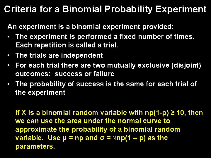
Criteria for a Binomial Probability Experiment An experiment is a binomial experiment provided: • The experiment is performed a fixed number of times. Each repetition is called a trial. • The trials are independent • For each trial there are two mutually exclusive (disjoint) outcomes: success or failure • The probability of success is the same for each trial of the experiment If X is a binomial random variable with np(1 -p) ≥ 10, then we can use the area under the normal curve to approximate the probability of a binomial random variable. Use μ = np and σ = √np(1 – p) as the parameters.

Why use a Normal Apx? ● For example, if n = 1000, then P(X ≥ 700) = P(X = 700) + P(X = 701) + … + P(X = 1000) which is the sum of 301 terms ● Each P(X = x) by itself is an involved calculation, and we need to do this 301 times, so this becomes an extremely long and tedious sum to compute! ● However, we can simplify this calculation ● As the number of trials, n, increases, then the distribution of binomial random variables becomes more and more bell shaped ● As a rule of thumb, if np(1 -p) ≥ 10, then the distribution will be reasonably bell shaped

Continuity Correction To approximate a binomial (discrete random variable) with a normal (continuous random variable) we add and subtract 0. 5 from our discrete value to convert to a continuous value.

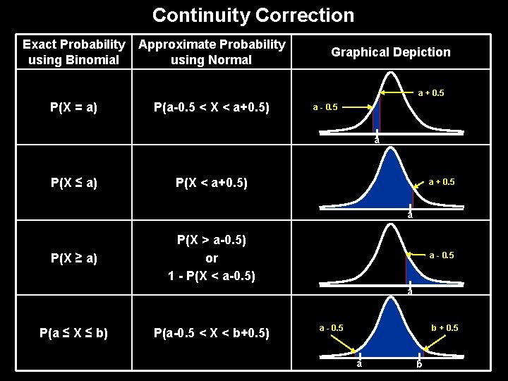
Continuity Correction Exact Probability Approximate Probability using Binomial using Normal Graphical Depiction a + 0. 5 P(X = a) P(a-0. 5 < X < a+0. 5) a - 0. 5 a P(X ≤ a) P(X < a+0. 5) a + 0. 5 a P(X ≥ a) P(X > a-0. 5) or 1 - P(X < a-0. 5) a - 0. 5 a P(a ≤ X ≤ b) P(a-0. 5 < X < b+0. 5) a - 0. 5 b + 0. 5 a b

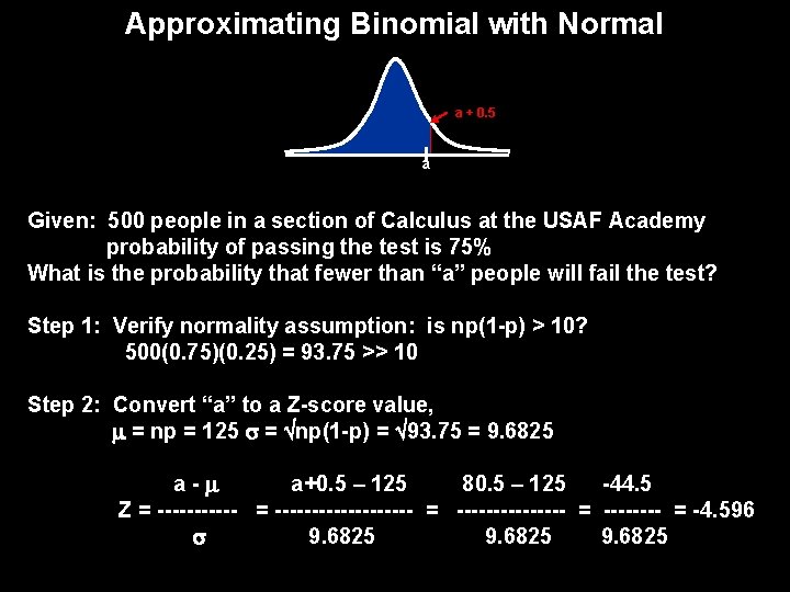
Approximating Binomial with Normal a + 0. 5 a Given: 500 people in a section of Calculus at the USAF Academy probability of passing the test is 75% What is the probability that fewer than “a” people will fail the test? Step 1: Verify normality assumption: is np(1 -p) > 10? 500(0. 75)(0. 25) = 93. 75 >> 10 Step 2: Convert “a” to a Z-score value, = np = 125 = np(1 -p) = 93. 75 = 9. 6825 a - a+0. 5 – 125 80. 5 – 125 -44. 5 Z = ---------- = -------- = -4. 596 9. 6825

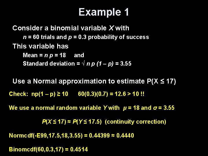
Example 1 Consider a binomial variable X with n = 60 trials and p = 0. 3 probability of success This variable has Mean = n p = 18 and Standard deviation = √ n p (1 – p) = 3. 55 Use a Normal approximation to estimate P(X ≤ 17) Check: np(1 – p) ≥ 10 60(0. 3)(0. 7) = 12. 6 > 10 !! We use a normal random variable Y with μ = 18 and σ = 3. 55 P(X ≤ 17) ≈ P(Y ≤ 17. 5) (continuity correction) Normcdf(-E 99, 17. 5, 18, 3. 55) = 0. 44399 ≈ 0. 4440 Binomcdf(60, 0. 3, 17) = 0. 4514

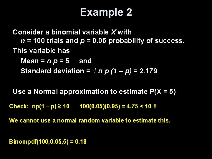
Example 2 Consider a binomial variable X with n = 100 trials and p = 0. 05 probability of success. This variable has Mean = n p = 5 and Standard deviation = √ n p (1 – p) = 2. 179 Use a Normal approximation to estimate P(X = 5) Check: np(1 – p) ≥ 10 100(0. 05)(0. 95) = 4. 75 < 10 !! We cannot use a normal random variable to estimate this. Binompdf(100, 0. 05, 5) = 0. 18

Summary and Homework • Summary – The binomial distribution is approximately bell shaped for large enough values of np(1 – p) – The normal distribution, with the same mean and standard deviation, can be used to approximate this binomial distribution – With technology, however, this approximation is not as needed as it used to be • Homework – pg 406 – 407; 5 – 7, 15, 21, 28