Lesson 7 1 Properties of the Normal Distribution

Lesson 7 - 1 Properties of the Normal Distribution

Quiz • Homework Problem: Chapter 6 review The number of cars that arrive at a bank’s window between 3: 00 pm and 6 pm on Friday follows a Poisson process at the rate of 0. 41 car every minute. Compute the possibility that the number of cars that arrive at the bank between 4: 00 pm and 4: 10 pm is a) exactly four cars b) fewer than four cars c) at least four cars • Reading questions: – What does the area under the graph represent in a continuous PDF? – What is the standard normal distribution variable called?

Objectives • Understand the uniform probability distribution • Graph a normal curve • State the properties of the normal curve • Understand the role of area in the normal density function • Understand the relationship between a normal random variable and a standard normal random variable

Vocabulary • Continuous random variable – has infinitely many values • Uniform probability distribution – probability distribution where the probability of occurrence is equally likely for any equal length intervals of the random variable X • Normal curve – bell shaped curve • Normal distributed random variable – has a PDF or relative frequency histogram shaped like a normal curve • Standard normal – normal PDF with mean of 0 and standard deviation of 1 (a z statistic!!)

Uniform PDF ● Sometimes we want to model a random variable that is equally likely between two limits ● When “every number” is equally likely in an interval, this is a uniform probability distribution – Any specific number has a zero probability of occurring – The mathematically correct way to phrase this is that any two intervals of equal length have the same probability ● Examples § Choose a random time … the number of seconds past the minute is random number in the interval from 0 to 60 § Observe a tire rolling at a high rate of speed … choose a random time … the angle of the tire valve to the vertical is a random number in the interval from 0 to 360

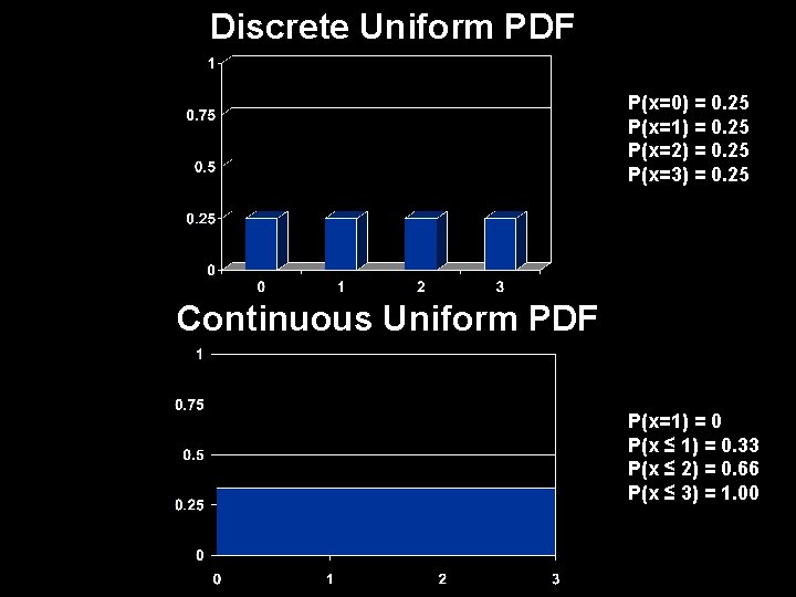
Discrete Uniform PDF P(x=0) = 0. 25 P(x=1) = 0. 25 P(x=2) = 0. 25 P(x=3) = 0. 25 Continuous Uniform PDF P(x=1) = 0 P(x ≤ 1) = 0. 33 P(x ≤ 2) = 0. 66 P(x ≤ 3) = 1. 00

Probability in a Continuous Probability Distributions Let P(x) denote the probability that the random variable X equals x, then 1) ∑ P(x) = 1 (sum of all probabilities must equal 1) → total area under the PDF graph must equal 1 2) The probability of x occurring in any interval, P(x), must between 0 and 1 0 ≤ P(x) ≤ 1 → the height of the graph of the PDF must be greater than or equal to 0 for all possible values of the random variable 3) The area underneath probability density function over some interval represents the probability of observing a value of the random variable in that interval.

Properties of the Normal Density Curve • It is symmetric about its mean, μ • Because mean = median = mode, the highest point occurs at x = μ • It has inflection points at μ – σ and μ + σ • Area under the curve = 1 • Area under the curve to the right of μ equals the area under the curve to the left of μ, which equals ½ • As x increases or decreases without bound (gets farther away from μ), the graph approaches, but never reaches the horizontal axis (like approaching an asymptote) • The Empirical Rule applies

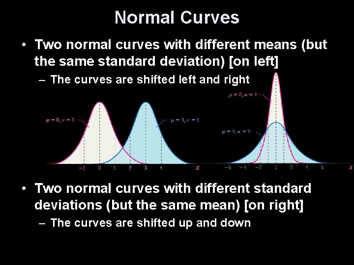
Normal Curves • Two normal curves with different means (but the same standard deviation) [on left] – The curves are shifted left and right • Two normal curves with different standard deviations (but the same mean) [on right] – The curves are shifted up and down

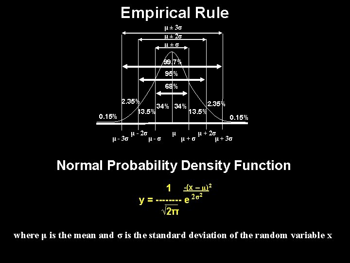
Empirical Rule μ ± 3σ μ ± 2σ μ±σ 99. 7% 95% 68% 0. 15% 2. 35% 34% 13. 5% μ - 3σ μ - 2σ μ-σ μ μ+σ 0. 15% μ + 2σ μ + 3σ Normal Probability Density Function 1 -(x – μ)2 2 y = ---- e 2σ √ 2π where μ is the mean and σ is the standard deviation of the random variable x

Area under a Normal Curve The area under the normal curve for any interval of values of the random variable X represents either • The proportion of the population with the characteristic described by the interval of values or • The probability that a randomly selected individual from the population will have the characteristic described by the interval of values [the area under the curve is either a proportion or the probability]

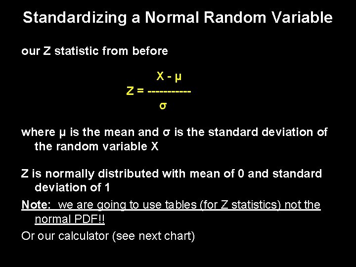
Standardizing a Normal Random Variable our Z statistic from before X-μ Z = -----σ where μ is the mean and σ is the standard deviation of the random variable X Z is normally distributed with mean of 0 and standard deviation of 1 Note: we are going to use tables (for Z statistics) not the normal PDF!! Or our calculator (see next chart)

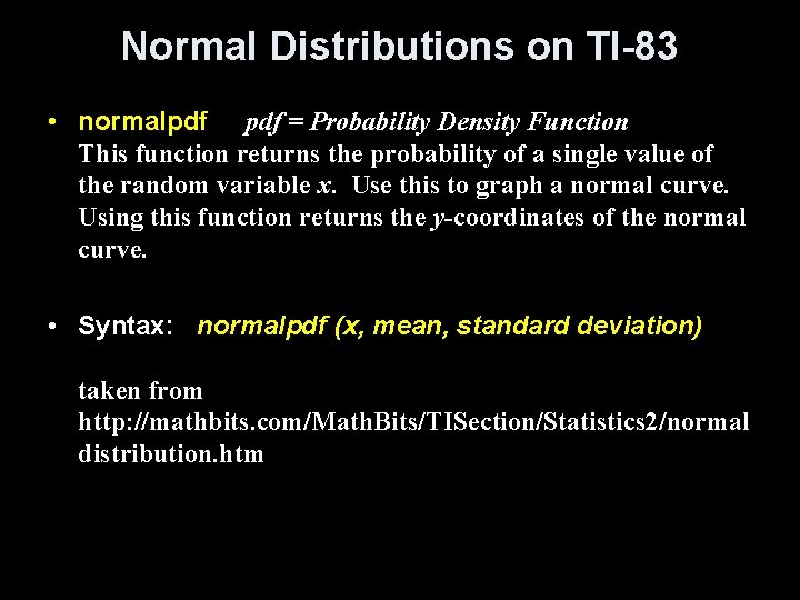
Normal Distributions on TI-83 • normalpdf = Probability Density Function This function returns the probability of a single value of the random variable x. Use this to graph a normal curve. Using this function returns the y-coordinates of the normal curve. • Syntax: normalpdf (x, mean, standard deviation) taken from http: //mathbits. com/Math. Bits/TISection/Statistics 2/normal distribution. htm

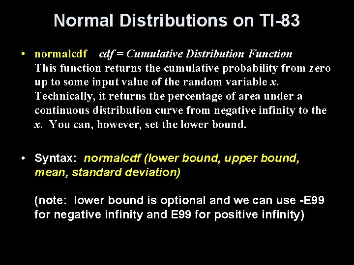
Normal Distributions on TI-83 • normalcdf = Cumulative Distribution Function This function returns the cumulative probability from zero up to some input value of the random variable x. Technically, it returns the percentage of area under a continuous distribution curve from negative infinity to the x. You can, however, set the lower bound. • Syntax: normalcdf (lower bound, upper bound, mean, standard deviation) (note: lower bound is optional and we can use -E 99 for negative infinity and E 99 for positive infinity)

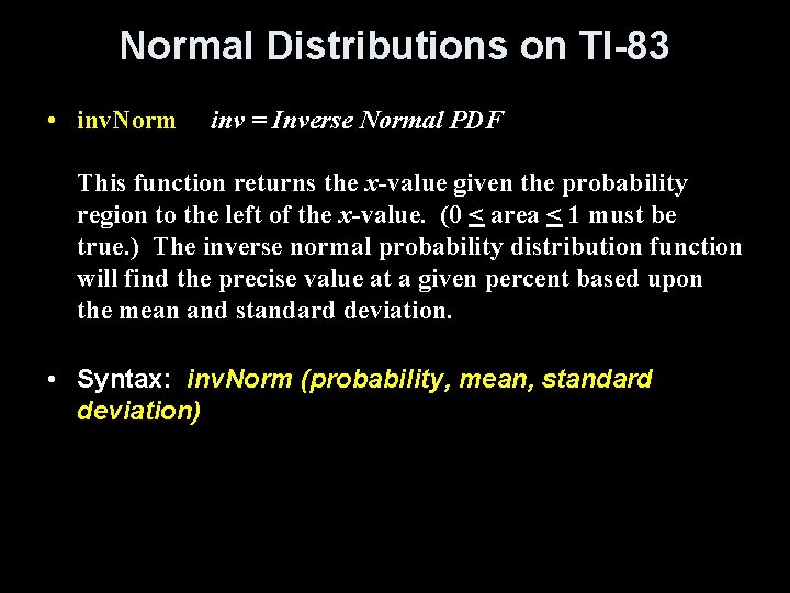
Normal Distributions on TI-83 • inv. Norm inv = Inverse Normal PDF This function returns the x-value given the probability region to the left of the x-value. (0 < area < 1 must be true. ) The inverse normal probability distribution function will find the precise value at a given percent based upon the mean and standard deviation. • Syntax: inv. Norm (probability, mean, standard deviation)

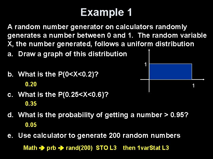
Example 1 A random number generator on calculators randomly generates a number between 0 and 1. The random variable X, the number generated, follows a uniform distribution a. Draw a graph of this distribution 1 b. What is the P(0<X<0. 2)? 0. 20 1 c. What is the P(0. 25<X<0. 6)? 0. 35 d. What is the probability of getting a number > 0. 95? 0. 05 e. Use calculator to generate 200 random numbers Math prb rand(200) STO L 3 then 1 var. Stat L 3

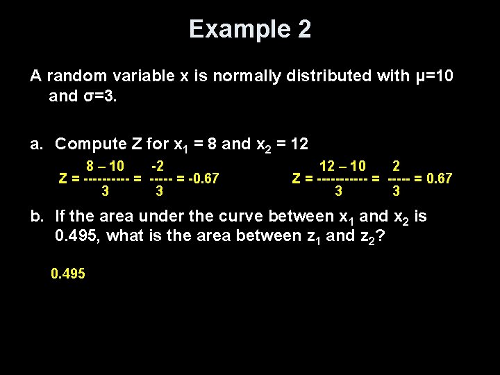
Example 2 A random variable x is normally distributed with μ=10 and σ=3. a. Compute Z for x 1 = 8 and x 2 = 12 8 – 10 -2 Z = ----- = -0. 67 3 3 12 – 10 2 Z = ------ = 0. 67 3 3 b. If the area under the curve between x 1 and x 2 is 0. 495, what is the area between z 1 and z 2? 0. 495

Summary and Homework • Summary – Normal probability distributions can be used to model data that have bell shaped distributions – Normal probability distributions are specified by their means and standard deviations – Areas under the curve of general normal probability distributions can be related to areas under the curve of the standard normal probability distribution • Homework – pg 367 – 371; 7 – 12; 15 -16, 19 -20, 32 -33